Pytorch Representation Learning: Part One
Project && Guide
Table of Contents
- Overview
- Contents
- Data
- Section 1. The Torch Tensor Library and Basic Operations
- 1.1. Import Libraries
- 1.2. Initialize a Random Tensor
- 1.3. Uniform Distribution Sampling
- 1.4. Get Tensor Shape
- 1.5. Tensor Types
- 1.6. Creation from Lists & Numpy
- 1.7. Simple Mathematical Operations
- 1.8. Broadcasting
- 1.9. Reshape
- 1.10. Repeat
- 1.11. Concatenate
- 1.12. Advanced Indexing
- 1.13. GPU Support
- 1.14. Move Tensors CPU <-> GPU
- 1.15. Contiguity in Memory
- Section 2. Autograd
- Section 3. Introduction to the Torch Neural Network Library
- Resources
- Project repository
Overview
This project is a hands-on curriculum for learning representation learning and deep learning with PyTorch. It includes a series of Jupyter Notebooks and Python scripts that guide you from basic tensor operations to advanced neural network architectures and generative models. Each section is designed to build practical skills, with real code examples and exercises covering:
- PyTorch fundamentals and tensor operations
- Automatic differentiation and autograd
- Neural network construction and training
- Convolutional and residual networks for image tasks
- Neural Machine Translation or Sequence models for machine translation
- Generative Adversarial Networks (GANs)
- Custom module creation and practical examples
The project is suitable for students, researchers, and practitioners who want to deepen their understanding of modern deep learning techniques through practical coding and experimentation.
Contents
- Section 1. The Torch Tensor Library and Basic Operations: Introduction to PyTorch tensors and basic operations.
- Section 2. Autograd: Understanding automatic differentiation and gradient computation in PyTorch.
- Section 3. Introduction to the Torch Neural Network Library: Building neural networks using PyTorch’s
nnmodule. - Section 4. Image Classification with Convnets and ResNets: Implementing convolutional neural networks (CNNs) and residual networks (ResNets) for image classification tasks.
- Section 5. Neural Machine Translation: Sequence-to-sequence models for translating text between languages.
- Section 6. Generative Adversarial Networks: Introduction to GANs and their applications.
- Section A. Creating Your Own Modules: Custom module creation in PyTorch.
- MNIST_example.py: Example script for training and evaluating models on the MNIST dataset.
Data
The data files of this project support experiments in:
- Neural machine translation (NMT) between Japanese and English
- Image classification using the MNIST dataset
Preprocessed files speed up training, while raw files allow for custom preprocessing and experimentation.
- jpn-dev.txt, jpn-test.txt, jpn-train.txt: Text files for Japanese-English neural machine translation. Used for training, validation, and testing models in the NMT notebook.
- nmt_license.txt: License information for the NMT dataset.
- processed/: Contains preprocessed PyTorch tensor files (
test.pt,training.pt) for efficient loading during model training and evaluation. - raw/: Contains original MNIST image and label files (
t10k-images-idx3-ubyte,t10k-labels-idx1-ubyte,train-images-idx3-ubyte,train-labels-idx1-ubyte) used for image classification tasks.
Section 1. The Torch Tensor Library and Basic Operations
1.1. Import Libraries
1
2
3
import numpy as np
from __future__ import print_function
import torch
Imports NumPy for array operations, enables print function compatibility, and imports PyTorch.
1.2. Initialize a Random Tensor
1
torch.Tensor(5, 3)
Creates a 5x3 tensor with uninitialized values.
1.3. Uniform Distribution Sampling
1
2
print(torch.Tensor(5, 3).uniform_(-1, 1))  # initialization
print(torch.rand(5,3)*2-1)                 # sampling
Initializes a tensor with values from a uniform distribution and samples random values in [-1, 1].
1.4. Get Tensor Shape
1
2
3
4
5
x = torch.Tensor(5, 3).uniform_(-1, 1)
print(x.size())      # shape
print(x.shape)       # shape (numpy style)
print(x.size(0))     # size of 0th axis
print(x.shape[0])    # size of 0th axis
Shows how to get tensor shape and dimensions.
1.5. Tensor Types
See the notebook for a table of tensor types (FloatTensor, LongTensor, etc.).
1.6. Creation from Lists & Numpy
1
2
3
4
5
z = torch.LongTensor([[1, 3], [2, 9]])
print(z.type())
print(z.numpy().dtype)
z_ = torch.LongTensor([[1, 3], [2, 9]])
z+z_
Creates tensors from lists, checks types, and adds tensors.
1
2
3
print(torch.from_numpy(np.random.rand(5, 3)).type())
print(torch.from_numpy(np.random.rand(5, 3).astype(np.float32)).type())
print(torch.from_numpy(np.random.rand(5, 3)).float().dtype)
Creates tensors from NumPy arrays and checks types.
1
a = torch.randn(1) # x ~ N(0,1)
Demonstrates type compatibility between tensors and NumPy arrays.
1.7. Simple Mathematical Operations
1
2
y = x ** torch.randn(5, 3)
print(y)
Element-wise exponentiation.
1
2
3
4
5
noise = torch.randn(5, 3)
1. Open the Jupyter Notebooks in your preferred environment (e.g., VS Code, Jupyter Lab).
2. Follow the notebooks in order for a structured learning path, or jump to specific topics as needed.
print(y)
print(y_)
Element-wise division and absolute value.
1.8. Broadcasting
1
2
3
4
print(x.size())
print(x)
y = x + torch.arange(3)
print(y)
Demonstrates broadcasting in tensor addition.
1.9. Reshape
1
2
3
4
5
6
7
8
9
y = torch.randn(5, 10, 15)
print(y.size())
print(y.view(-1, 15).size())
print(y.view(-1, 15).unsqueeze(1).size())
print(y.view(-1, 15).unsqueeze(1).unsqueeze(2).unsqueeze(3).squeeze().size())
print(y.transpose(0, 1).size())
print(y.transpose(1, 2).size())
print(y.transpose(0, 1).transpose(1, 2).size())
print(y.permute(1, 2, 0).size())
Shows reshaping, unsqueezing, squeezing, transposing, and permuting tensors.
1.10. Repeat
1
2
3
print(y.view(-1, 15).unsqueeze(1).expand(50, 100, 15).size())
print(y.view(-1, 15).unsqueeze(1).expand_as(torch.randn(50, 100, 15)).size())
print(y.view(-1, 15).unsqueeze(1).repeat(50,100,1).size())
Demonstrates expanding and repeating tensors.
1.11. Concatenate
1
2
3
print(torch.cat([y, y], 2).size())
print(torch.stack([y, y], 0).size())
print(torch.cat([y[None], y[None]], 0).size())
Concatenates and stacks tensors along different dimensions.
1.12. Advanced Indexing
1
2
3
4
5
6
7
8
9
y = torch.randn(2, 3, 4)
print(y[[1, 0, 1, 1]].size())
rev_idx = torch.arange(1, -1, -1).long()
print(rev_idx)
print(y[rev_idx].size())
3. Use `MNIST_example.py` for a standalone example of model training and evaluation.
print(v.shape)
print(v)
print(torch.gather(v, 1, torch.tensor([1,2,0]).long().unsqueeze(1)))
Shows advanced indexing and gathering elements.
1.13. GPU Support
1
x = torch.cuda.HalfTensor(5, 3).uniform_(-1, 1)
Demonstrates tensor operations on GPU.
1.14. Move Tensors CPU <-> GPU
1
2
3
4
5
6
x = torch.FloatTensor(5, 3).uniform_(-1, 1)
print(x)
- Python 3.x
print(x)
- PyTorch
print(x)
Moves tensors between CPU and GPU.
1.15. Contiguity in Memory
1
2
3
4
5
6
x = torch.FloatTensor(5, 3).uniform_(-1, 1)
print(x)
print('Contiguity : %s ' % (x.is_contiguous()))
x = x.unsqueeze(0).expand(30, 5, 3)
print('Contiguity : %s ' % (x.is_contiguous()))
print('Contiguity : %s ' % (x.is_contiguous()))
Checks and ensures tensor contiguity in memory.
Section 2. Autograd
Variables : Thin wrappers around tensors to facilitate autograd
Variables in PyTorch are now just tensors with autograd support. They support almost all operations that can be performed on regular tensors.
2.1. Properties of Tensor : Requiring gradients, Data & Grad
- You can access the raw tensor through the .data attribute
- Gradient of the loss w.r.t. this variable is accumulated into .grad.
- Stay tuned for requires_grad
1
2
3
4
5
z = torch.Tensor(5, 3).uniform_(-1, 1)
print(z.data)
print('Gradient : %s ' % (z.grad))
print('Requires Gradient : %s ' % (z.requires_grad))
print('Requires Gradient : %s ' % (z.requires_grad_().requires_grad))
Shows how to access the raw tensor, check gradients, and set requires_grad.
2.2. Define-by-run Paradigm
The torch autograd package provides automatic differentiation for all operations on Tensors.
PyTorch’s autograd is a reverse mode automatic differentiation system.
Backprop is defined by how your code is run, and that every single iteration can be different.
Other frameworks that adopt a similar approach :
How autograd encodes execution history
Autograd maintains a graph that records all operations performed on tensors. This graph is recreated from scratch at every iteration, allowing for dynamic computation graphs.
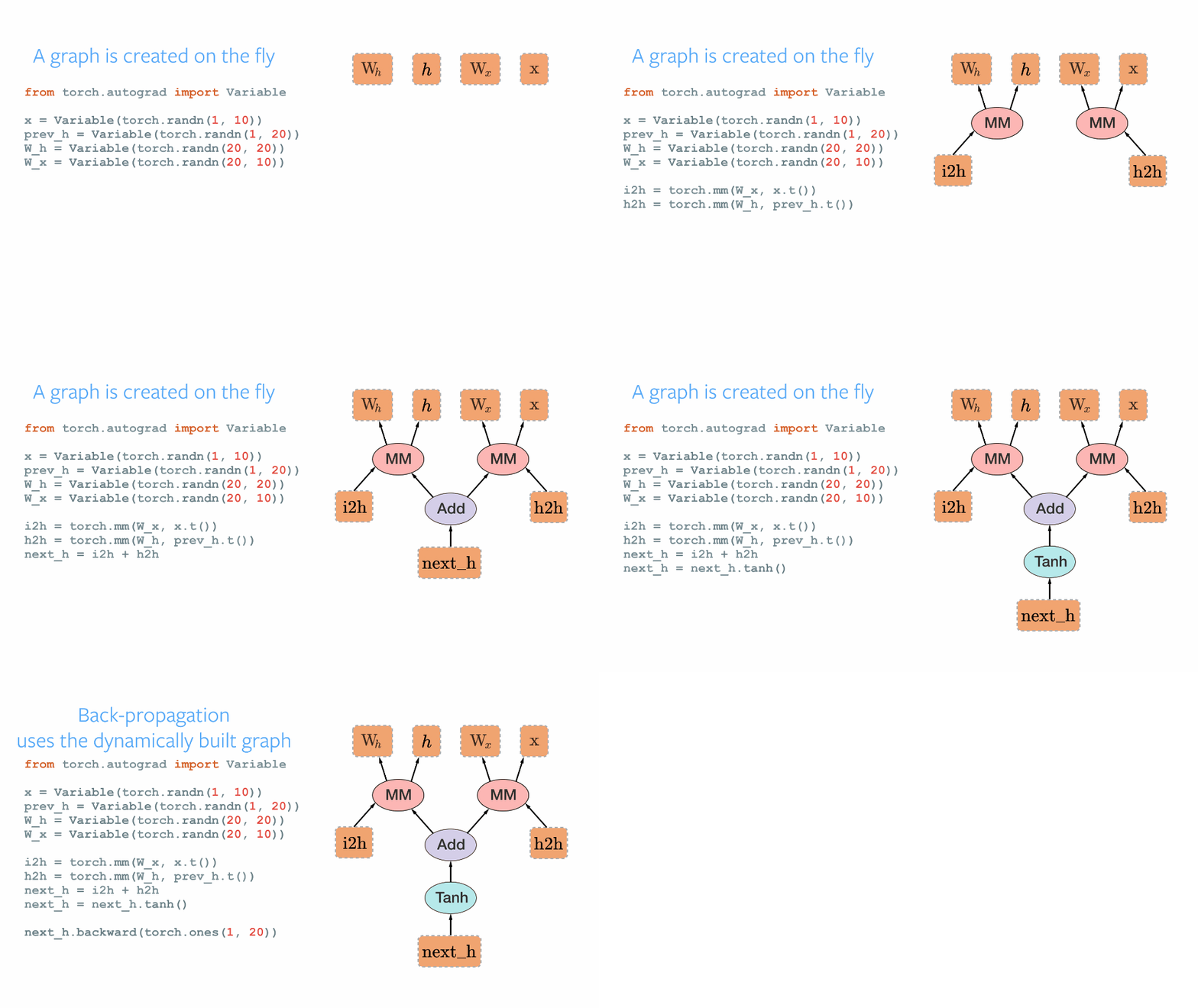 [GIF source]:(https://github.com/pytorch/pytorch)
Inside PyTorch, autograd builds a graph made of Function objects (expressions) that can be applied to evaluate results. As the forward pass runs, autograd both performs calculations and constructs a graph describing how to compute gradients. Each Variable’s .grad_fn attribute points to this graph. After the forward pass, the graph is used in the backward pass to calculate gradients.
1
2
3
4
x = torch.Tensor(5, 3).uniform_(-1, 1)
y = torch.Tensor(3, 5).uniform_(-1, 1)
z = torch.mm(x, y)
print(z.grad_fn)
Shows the grad_fn attribute, which is the entry point into the computation graph.
Getting gradients : backward() & torch.autograd.grad
1
2
3
4
5
6
7
8
9
10
x = torch.Tensor(5, 3).uniform_(-1, 1).requires_grad_()
y = torch.Tensor(5, 3).uniform_(-1, 1).requires_grad_()
z = x ** 2 + 3 * y
print(z.grad_fn)
z.sum().backward()
print(x.grad)
torch.eq(x.grad, 2 * x)
y.grad
dz_dx = torch.autograd.grad(z, x, grad_outputs=torch.ones(5, 3))
dz_dy = torch.autograd.grad(z, y, grad_outputs=torch.ones(5, 3))
Demonstrates both backward() and torch.autograd.grad for computing gradients.
2.3. Define-by-run example
Common Variable definition
1
2
3
x = torch.Tensor(5, 3).uniform_(-1, 1).requires_grad_()
w = torch.Tensor(3, 10).uniform_(-1, 1).requires_grad_()
b = torch.Tensor(10,).uniform_(-1, 1).requires_grad_()
Graph 1 : wx + b
1
2
3
4
5
6
o = torch.matmul(x, w) + b
do_dinputs_1 = torch.autograd.grad(o, [x, w, b], grad_outputs=torch.ones(5, 10))
print('Gradients of o w.r.t inputs in Graph 1')
print('do/dx : \n\n %s ' % (do_dinputs_1[0]))
print('do/dw : \n\n %s ' % (do_dinputs_1[1]))
print('do/db : \n\n %s ' % (do_dinputs_1[2]))
Graph 2 : wx / b
1
2
3
4
5
6
o = torch.matmul(x, w) / b
do_dinputs_2 = torch.autograd.grad(o, [x, w, b], grad_outputs=torch.ones(5, 10))
print('Gradients of o w.r.t inputs in Graph 2')
print('do/dx : \n %s ' % (do_dinputs_2[0]), (w/b[None,:]).sum(1))
print('do/dw : \n %s ' % (do_dinputs_2[1]), (x.sum(0)[:,None]/b[None,:]))
print('do/db : \n %s ' % (do_dinputs_2[2]))
2.4. Gradient buffers: .backward() and retain_graph=True
- Calling
.backward()clears the current computation graph. - Once
.backward()is called, intermediate variables used in the construction of the graph are removed. - This is used implicitly to let PyTorch know when a new graph is to be built for a new minibatch. This is built around the forward and backward pass paradigm.
- To retain the graph after the backward pass use
loss.backward(retain_graph=True). This lets you re-use intermediate variables to potentially compute a secondary loss after the initial gradients are computed. This is useful to implement things like the gradient penalty in WGANs (https://arxiv.org/abs/1704.00028)
1
2
3
4
5
6
7
o = torch.mm(x, w) + b
o.backward(torch.ones(5, 10))
# Call backward again -> This fails
o = torch.mm(x, w) + b
o.backward(torch.ones(5, 10), retain_graph=True)
o = o ** 3
o.backward(torch.ones(5, 10))
WARNING: Calling .backward() multiple times will accumulate gradients into .grad and NOT overwrite them.
1
2
3
4
5
6
7
8
9
10
11
12
13
x = torch.Tensor(5, 3).uniform_(-1, 1).requires_grad_()
w = torch.Tensor(3, 10).uniform_(-1, 1).requires_grad_()
b = torch.Tensor(10,).uniform_(-1, 1).requires_grad_()
print(b.grad)
o = torch.mm(x, w) + b
o.backward(torch.ones(5, 10), retain_graph=True)
print(b.grad)
o.backward(torch.ones(5, 10), retain_graph=True)
print(b.grad)
# ...repeated calls accumulate gradients
for i in range(100):
	o.backward(torch.ones(5, 10), retain_graph=True)
print(b.grad)
Excluding subgraphs from backward: requires_grad=False, volatile=True & .detach
-
If there’s a single input to an operation that requires gradient, its output will also require gradient.
-
Conversely, if all inputs don’t require gradient, the output won’t require it.
-
Backward computation is never performed in the subgraphs where all Variables didn’t require gradients.
-
This is potentially useful when you have part of a network that is pretrained and not fine-tuned, for example word embeddings or a pretrained imagenet model.
requires_grad=False
1
2
3
4
5
6
7
x = torch.Tensor(3, 5).uniform_(-1, 1).requires_grad_(False)
y = torch.Tensor(3, 5).uniform_(-1, 1).requires_grad_(False)
z = torch.Tensor(3, 5).uniform_(-1, 1).requires_grad_(True)
o = x + y
print(' o = x + y requires grad ? : %s ' % (o.requires_grad))
o = x + y + z
print(' o = x + y + z requires grad ? : %s ' % (o.requires_grad))
.detach()
- It is possible to detach variables from the graph by calling
.detach(). - This could lead to disconnected graphs. In which case PyTorch will only backpropagate gradients until the point of disconnection.
1
2
3
4
5
6
7
8
9
10
11
x = torch.Tensor(3, 5).uniform_(-1, 1).requires_grad_()
y = torch.Tensor(3, 5).uniform_(-1, 1).requires_grad_()
z = torch.Tensor(3, 5).uniform_(-1, 1).requires_grad_()
m1 = x + y
m2 = z ** 2
m1 = m1.detach()
m3 = m1 + m2
m3.backward(torch.ones(3, 5))
print('dm3/dx \n\n %s ' % (x.grad))
print('\ndm3/dy \n\n %s ' % (y.grad))
print('\ndm3/dz \n\n %s ' % (z.grad))
2.5 Gradients w.r.t intermediate variables in the graph
To compute gradients w.r.t intermediate variables, use .retain_grad() or explicitly compute gradients using torch.autograd.grad.
-
By default, all PyTorch gradient computations w.r.t intermediate nodes in the graph are ad-hoc.
-
This is in the interest of saving memory.
-
To compute gradients w.r.t intermediate variables, use
.retain_grad()or explicitly compute gradients usingtorch.autograd.grad -
.retain_grad()populates the.gradattribute of the Variable whiletorch.autograd.gradreturns a Variable that contains the gradients.
1
2
3
4
5
6
7
8
9
10
11
x = torch.Tensor(3, 5).uniform_(-1, 1).requires_grad_()
y = torch.Tensor(3, 5).uniform_(-1, 1).requires_grad_()
z = torch.Tensor(3, 5).uniform_(-1, 1).requires_grad_()
m1 = x + y
m2 = z ** 2
m1.retain_grad()
m2.retain_grad()
m3 = m1 * m2
m3.backward(torch.ones(3, 5))
print('dm3/dm1 \n\n %s ' % (m1.grad))
print('dm3/dm2 \n\n %s ' % (m2.grad))
In place operations with autograd
In-place operations are suffixed by _ (e.g., log_, uniform_). Supporting in-place operations in autograd is difficult and PyTorch discourages their use in most cases. They can overwrite values required to compute gradients and complicate the computation graph.
In-place operations in PyTorch are limited because:
They can overwrite values needed for gradient computation, making some gradients unstable or hard to recover. They require rewriting the computational graph, which is complex and error-prone, especially when multiple variables share the same storage. This can lead to errors if modified storage is referenced elsewhere.
Second and higher order derivatives
2.6. Computing gradients w.r.t gradients
1
2
3
4
5
6
7
8
9
10
x = torch.Tensor(5, 3).uniform_(-1, 1).requires_grad_()
y = torch.Tensor(3, 5).uniform_(-1, 1).requires_grad_()
z = torch.Tensor(5, 5).uniform_(-1, 1).requires_grad_()
o = torch.mm(x, y) + z ** 2
#do_dz = torch.autograd.grad(o, z, grad_outputs=torch.ones(5, 5), retain_graph=True, create_graph=True)
do_dz = torch.autograd.grad(o, z, grad_outputs=torch.ones(5, 5), retain_graph=True)
print('do/dz \n\n : %s ' % (do_dz[0]))
l = o + do_dz[0]
dl_dz = torch.autograd.grad(l, z, grad_outputs=torch.ones(5, 5))
print('dl/dz \n\n : %s ' % (dl_dz[0]))
Shows how to compute higher order derivatives, useful for gradient penalty (e.g., WGAN-GP).
Section 3. Introduction to the Torch Neural Network Library
3.1. torch.nn
Neural networks can be constructed using the torch.nn package, which provides all neural network related functionalities.
1
2
3
4
5
import torch
import torch.nn as nn
import torch.optim as optim
import torch.nn.init as init
import torch.nn.functional as F
3.2. Linear, Bilinear & Nonlinearities
1
2
3
4
5
6
7
8
9
x = torch.randn(32, 10)
y = torch.randn(32, 30)
sigmoid = nn.Sigmoid()
linear = nn.Linear(in_features=10, out_features=20, bias=True)
output_linear = linear(x)
bilinear = nn.Bilinear(in1_features=10, in2_features=30, out_features=50, bias=True)
output_bilinear = bilinear(x, y)
print('Linear output size : ', output_linear.size())
print('Bilinear output size : ', output_bilinear.size())
Demonstrates linear, bilinear layers and nonlinearities like sigmoid.
3.3. Convolution, BatchNorm & Pooling Layers
1
2
3
4
5
6
7
x = torch.randn(10, 3, 28, 28)
conv = nn.Conv2d(in_channels=3, out_channels=32, kernel_size=(3, 3), stride=1, padding=1, bias=True)
pool = nn.MaxPool2d(kernel_size=(2, 2), stride=2)
output_conv = conv(x)
outpout_pool = pool(conv(x))
print('Conv output size : ', output_conv.size())
print('Pool output size : ', outpout_pool.size())
Shows convolution, batch normalization, and pooling layers.
3.4. Recurrent, Embedding & Dropout Layers
1
2
3
4
5
6
7
8
9
10
11
inputs = [[1, 2, 3], [1, 0, 4], [1, 2, 4], [1, 4, 0], [1, 3, 3]]
x = torch.LongTensor(inputs)
embedding = nn.Embedding(num_embeddings=5, embedding_dim=20, padding_idx=1)
drop = nn.Dropout(p=0.5)
rnn = nn.RNN(input_size=20, hidden_size=50, num_layers=2, batch_first=True, bidirectional=True, dropout=0.3)
emb = drop(embedding(x))
rnn_h, rnn_h_t = rnn(emb)
print('Embedding size : ', emb.size())
print('GRU hidden states size : ', rnn_h.size())
print('GRU last hidden state size : ', rnn_h_t.size())
print(emb[1,0])
Demonstrates embedding, dropout, and recurrent layers.
3.5. torch.nn.functional
Using the above classes requires defining an instance of the class and then running inputs through the instance.
The functional API provides a way to use layers and activations in a functional style. Such as
import torch.nn.functional as F
- Linear layers -
F.linear(input=x, weight=W, bias=b) - Convolution Layers -
F.conv2d(input=x, weight=W, bias=b, stride=1, padding=0, dilation=1, groups=1) - Nonlinearities -
F.sigmoid(x), F.tanh(x), F.relu(x), F.softmax(x) - Dropout -
F.dropout(x, p=0.5, training=True)
3.6. A few examples of the functional API
1
2
3
4
x = torch.randn(10, 3, 28, 28)
filters = torch.randn(32, 3, 3, 3)
conv_out = F.relu(F.dropout(F.conv2d(input=x, weight=filters, padding=1), p=0.5, training=True))
print('Conv output size : ', conv_out.size())
Shows functional API for convolution, dropout, and activation.
3.7. torch.nn.init
Provides functions for standard weight initialization techniques.
1
2
3
4
5
conv_layer = nn.Conv2d(in_channels=3, out_channels=32, kernel_size=(3, 3), padding=1)
for k,v in conv_layer.named_parameters():
    print(k)
    if k == 'weight':
        init.kaiming_normal_(v)
Shows how to initialize convolution kernels with Kaiming normal initialization.
3.8. torch.optim
Provides implementations of standard stochastic optimization techniques.
1
2
3
4
W1 = torch.randn(10, 20, requires_grad=True)
W2 = torch.randn(10, 20, requires_grad=True)
optimizer = optim.SGD([W1, W2], lr=0.01, momentum=0.9, dampening=0, weight_decay=1e-2, nesterov=True)
optimizer = optim.Adam([W1, W2], lr=0.001, betas=(0.9, 0.999), eps=1e-08, weight_decay=0)
Shows SGD and Adam optimizers.
3.9. Learning Rate Scheduling
1
2
scheduler = optim.lr_scheduler.MultiStepLR(optimizer, milestones=[30,80], gamma=0.1)
scheduler = optim.lr_scheduler.ReduceLROnPlateau(optimizer, mode='min', factor=0.1, patience=10, verbose=True, threshold=1e-04, threshold_mode='rel', min_lr=1e-05, eps=1e-08)
Shows learning rate scheduling with MultiStepLR and ReduceLROnPlateau.
Resources
Project repository
GitHub Code: PyTorch Representation Learning Project