Signal Processing: 2D Signals and Image processing
Project && Guide
Table of Contents
- Overview
- Key Techniques and Concepts
- Section 1: Spatial filtering
- Section 2: Fourier Transform and Spectral Filtering
- Project repository
Overview
This document is a comprehensive guide to 2D signal and image processing, based on exercises and code from Analyze_2D_Signals.ipynb. It is structured to help students and practitioners understand, implement, and visualize key image processing techniques. The topics covered include:
- Spatial Filtering: Smoothing, sharpening, and denoising images using convolution, median, and Gaussian filters.
- Histogram Equalization: Enhancing image contrast and visual quality.
- Edge Detection and Enhancement: Using Laplacian and other filters to highlight image features.
- Morphological Operations: Binary image processing for object detection and counting (e.g., coin counter).
- Fourier Transform and Spectral Analysis: Understanding frequency domain properties, filtering, and spectral manipulation.
- Spectral and Homomorphic Filtering: Removing periodic noise and improving illumination/reflection balance in images.
Each section provides clear explanations, annotated code blocks, and visualizations to reinforce learning. The document is designed for practical use in image analysis projects, with step-by-step guidance for each technique.
Key Techniques and Concepts:
Section 1: Spatial filtering
Note: Pay attention to array datatypes (e.g., np.uint8, np.float32) for image processing. Use imshow with vmin/vmax for proper grayscale display.
1
plt.imshow(mon_img, vmin=0, vmax=255)
Note: Import required libraries
1
2
3
4
5
6
7
import cv2
import numpy as np
import matplotlib.pyplot as plt
plt.rcParams['image.cmap'] = 'gray'
import matplotlib
matplotlib.rcParams['figure.figsize'] = (15.0, 15.0)
from scipy.signal import medfilt2d
1.1: Image Quality Enhancement
1) Histogram Equalization
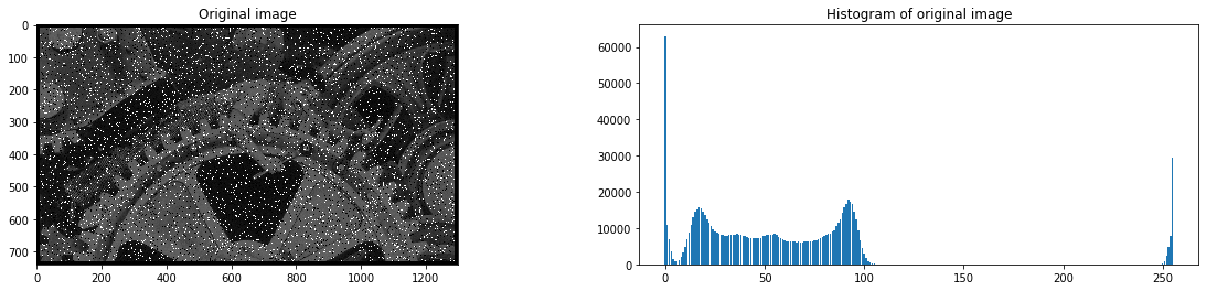
Load and display the image, plot its histogram, and apply histogram equalization.
1
2
3
4
5
6
7
8
9
10
11
12
13
14
15
16
17
18
19
20
21
22
23
24
25
26
27
28
29
30
31
32
33
34
35
36
37
38
39
40
41
42
43
44
45
46
# Functions for histogram plotting and equalization

# Plot the histogram of an image
# img: image as a np.ndarray, values between [0,255]
# ax: (optional) matplotlib axis for plotting
# title_txt: (optional) title for the histogram plot
def plot_histogram(img, ax=None, title_txt = None):
    """
    Plot the histogram of an image.
    img: image as a np.ndarray, values between [0,255]
    ax: (optional) matplotlib axis for plotting
    """
    hist, bins = np.histogram(img, 256,[0,256])
    if ax is not None:
        ax.bar(bins[:-1], hist)
        ax.set_title(title_txt)
    else:
        plt.bar(bins[:-1], hist)
        plt.title(title_txt)
    plt.show()
    return

# Perform histogram equalization on an image
# img: image as np.uint8
def equalize_histogram(img):
    """
    Perform histogram equalization on an image.
    img: image as np.uint8
    """
    hist, bins = np.histogram(img, 256,[0,256])
    hist = hist.astype(np.float32)
    T = hist.cumsum()  # Cumulative sum for equalization
    T_normalized= 255* (T - T.min())/(T.max()-T.min())  # Normalize
    eq_img=T_normalized[img]
    return eq_img.astype(np.uint8)

img1 = cv2.imread('TempsModernes.jpeg', cv2.IMREAD_GRAYSCALE)
fig1, (ax, ax1) = plt.subplots(1,2, figsize=(20,4))
ax.imshow(img1, vmin=0, vmax=255)
ax.set_title("Original image")
plot_histogram(img1,ax1, "Histogram of original image")
img2 = equalize_histogram(img1)
fig2, (ax, ax1) = plt.subplots(1,2, figsize=(20,4))
ax.imshow(img2, vmin=0, vmax=255)
ax.set_title("Histogram Equalized image")
plot_histogram(img2,ax1, "Histogram of equalized image")
Histogram equalization flattens the histogram and enhances image contrast.
2) Median Filtering
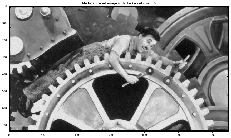
Salt and pepper noise is predominant. Median filter removes it while preserving edges.
1
2
3
4
kernel_size = 5
image_med = medfilt2d(img2, kernel_size)
plt.imshow(image_med, vmin=0, vmax=255)
plt.title("Median filtered image with the kernel size = {}".format(kernel_size))
3) 2D Convolution (Gaussian Smoothing)
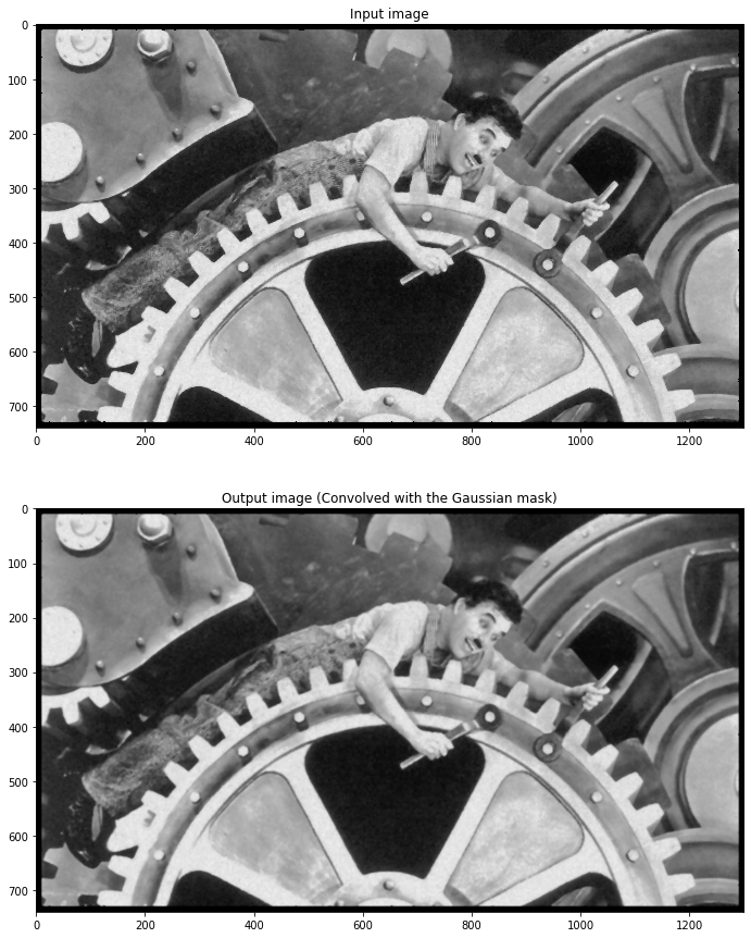
Implement conv2d and apply a Gaussian mask.
1
2
3
4
5
6
7
8
9
10
11
12
13
14
15
16
17
18
19
20
21
22
23
24
25
26
27
# Function for 2D convolution of an image with a mask
# img: input image as np.uint8
# mask: convolution mask (square, odd size)
def conv2d(img, mask):
    """
    Perform 2D convolution of an image with a mask.
    img: image as np.uint8
    mask: The mask to be convolved
    Returns: convolved image (same size as input)
    """
    out = np.zeros(img.shape, dtype=np.float32)  # Output image
    size_mask = mask.shape[0]  # Mask size
    pad_values = int((size_mask-1)/2)  # Amount of zero-padding
    img = np.pad(img, ((pad_values, pad_values), (pad_values, pad_values)))  # Pad image
    for i, row in enumerate(out):
        for j, col in enumerate(row):
            roi = img[i :i + size_mask , j : j + size_mask ]  # Region of interest
            out[i,j] = (roi * mask).sum()  # Convolution operation
    return out

mask = np.asarray([[1,2,1,2,1],[2,4,8,4,2],[1,8,18,8,1],[2,4,8,4,2],[1,2,1,2,1]])/90
img_med_conv=conv2d(image_med, mask)
fig, (ax, ax1) = plt.subplots(2,1)
ax.imshow(image_med, vmin=0, vmax=255)
ax.set_title("Input image")
ax1.imshow(img_med_conv, vmin=0, vmax=255)
ax1.set_title("Output image (Convolved with the Gaussian mask)")
Gaussian convolution smooths the image, making it slightly blurry.
4) Edge Enhancement (Laplacian)
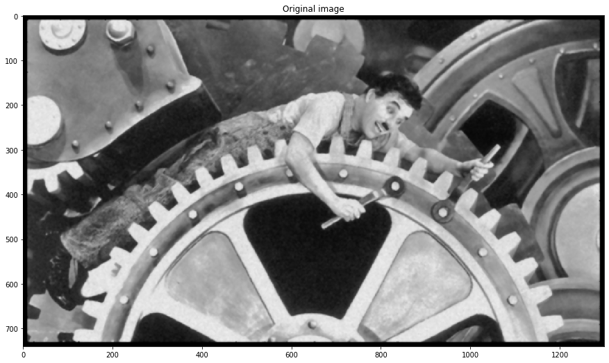
Apply Laplacian filter to enhance edges after smoothing.
1
2
3
4
5
6
7
8
mask_laplacian = np.asarray([[-1,-1,-1], [-1,8,-1], [-1,-1,-1]])
mask_gaussian = np.asarray([[1,2,1], [2,4,2], [1,2,1]])/16
I_g = conv2d(img_med_conv, mask_gaussian)
Delta_I_g=conv2d(I_g, mask_laplacian)
k = 1.5
I_r = I_g + k * Delta_I_g
plt.imshow(I_r, vmin=0, vmax=255)
plt.title("Enhanced image")
Combining Laplacian and Gaussian enhances edges; optimal k balances sharpness and smoothness.
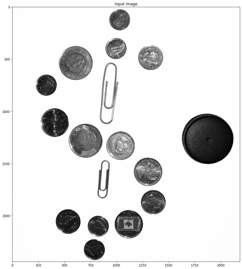
1.2: Coin counter
1) Load and Display Coins Image
1
2
3
img = cv2.imread('pieces.jpg', cv2.IMREAD_GRAYSCALE)
plt.imshow(img, vmin=0, vmax=255)
plt.title("Input image")
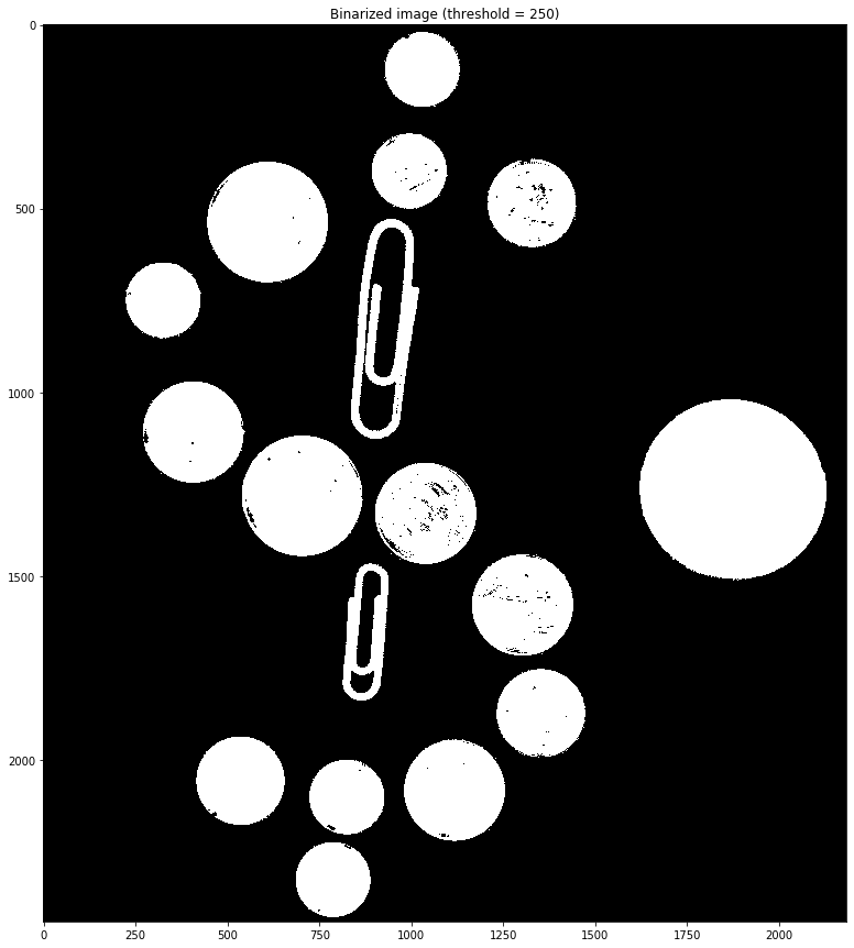
2) Binarization
Threshold and invert to highlight coins.
1
2
3
4
5
6
7
def binarize(img, threshold):
    img_binary = np.uint8(255*(img>threshold))
    return img_binary
threshold = 250
img_b = 255- binarize(img,threshold)
plt.imshow(img_b, vmin=0, vmax=255)
plt.title("Binarized image (threshold = {})".format(threshold))
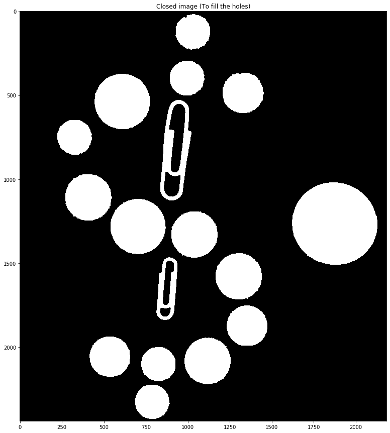
3) Morphological Closing
Fill holes in coins using elliptical kernel.
1
2
3
4
kernel = cv2.getStructuringElement(cv2.MORPH_ELLIPSE,(15,15))
img_close = cv2.morphologyEx(img_b, cv2.MORPH_CLOSE, kernel)
plt.imshow(img_close, vmin=0, vmax=255)
plt.title("Closed image (To fill the holes)")
4) Counting Coins
Use erosion and connected components to count coins and sum their value.
1
2
3
4
5
6
7
8
9
10
11
12
13
14
15
16
17
18
19
20
21
22
def nb_components(img_bin):
    num_labels, labels_im = cv2.connectedComponents(img_bin)
    return num_labels-1
coin_val = np.asarray([0, 10, 5, 25, 200])
stct_radius = np.asarray([90,110,120,140,200])
stct_diameter= 2 * stct_radius
list_nb_coins= []
totall_coins=nb_components(img_close)
for ind, i in enumerate(stct_diameter):
    kernel = cv2.getStructuringElement(cv2.MORPH_ELLIPSE,(i,i))
    img_erode = cv2.morphologyEx(img_close, cv2.MORPH_ERODE, kernel)
    nb_coins = nb_components(img_erode)
    dis_coins = totall_coins-nb_coins
    list_nb_coins.append(dis_coins)
    totall_coins = nb_coins
    c = coin_val[ind]%100
    d = coin_val[ind]//100
    print('Coin values: {} ($).{} (¢) --> Number of coins: {}'.format(d,c,dis_coins))
total_value = (list_nb_coins*coin_val).sum()
c_total = total_value%100
d_total = total_value//100
print('\nSummation:  {}($).{}(¢) '.format(d_total,c_total))
Section 2: Fourier Transform and Spectral Filtering
2.1: 2D Fast Fourier Transform (FFT)
FFT stands for Fast Fourier Transform. It is an efficient algorithm to compute the Discrete Fourier Transform (DFT) and its inverse. FFT transforms a signal from the time (or spatial) domain into the frequency domain, allowing you to analyze the frequency components present in the signal or image. In image processing, FFT is used to study patterns, filter noise, and perform spectral analysis.
The goal of this section is to familiarize yourself with the 2D-Fourier transform and some of its properties.
We are going to study the function: \(f(x, y) = \sin\left(\frac{2\pi}{256}[f_1 x+f_2 y]\right), \quad x, y \in [0, 256]\)
1) Generate 2D Sinusoidal Image
Create the function below, which takes ${f_1, f_2}$ as parameters and outputs a monochromatic image of size 256x256. Using np.meshgrid allows efficient array creation without explicit loops.
1
2
3
4
5
6
7
8
9
def f(f_i):
    f1 = f_i[0]
    f2 = f_i[1]
    # To get the image of size 256*256, x and y are in the range of 0 ..255
    x = np.arange(0,256)
    y = np.arange(0,256)
    xv, yv = np.meshgrid(x, y)
    f = np.sin(2*np.pi/256*(f1*xv+f2*yv))
    return f
This function generates a 2D sinusoidal pattern, where $f_1$ and $f_2$ control the frequency along the $x$ and $y$ axes, respectively. np.meshgrid efficiently creates coordinate matrices for vectorized computation.
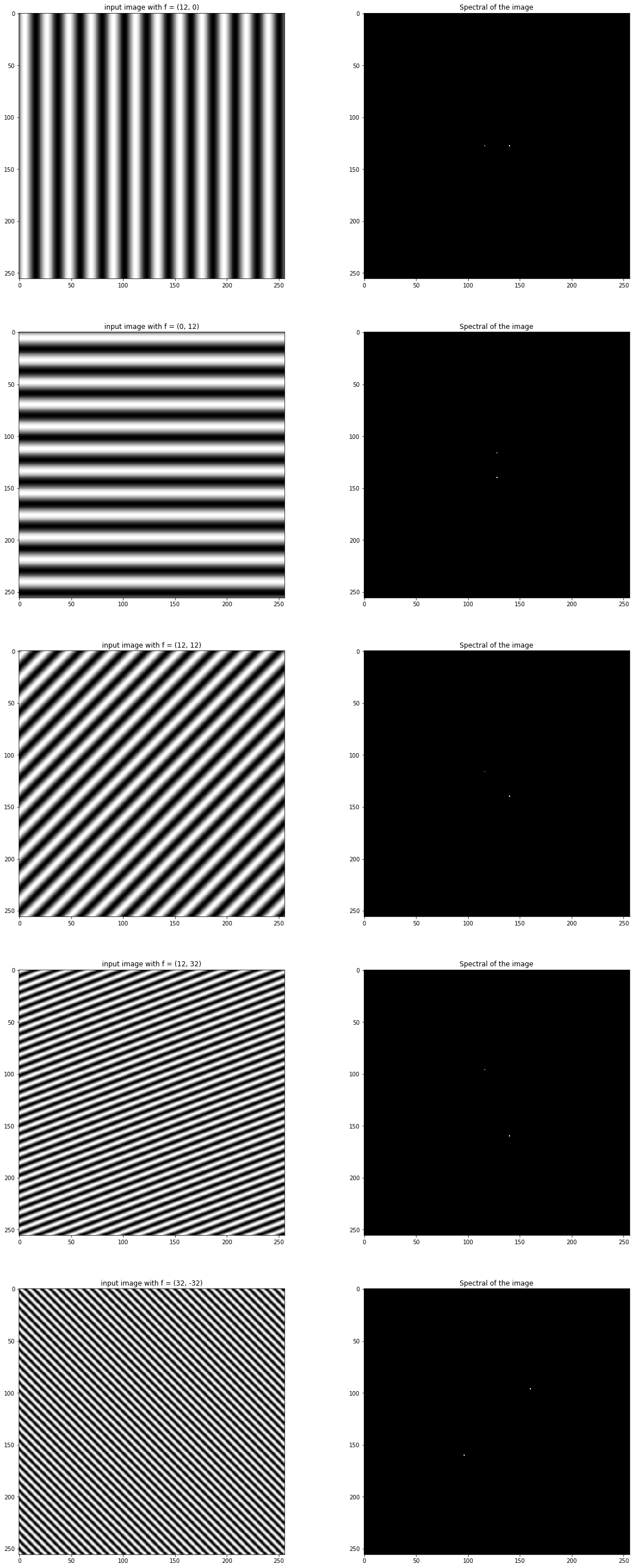
2) Visualize 2D FFT Spectrum
For each pair of parameters ${f_1, f_2}$, display the image $f(x, y)$ and its spectrum (amplitude of the Fourier Transform) side by side. The spectrum is computed and normalized so its maximum is 1 and minimum is 0.
The normalization formula is: \(f_{normalisée} = \frac{f-\min(f)}{\max(f)-\min(f)}\)
The function below computes the normalized spectrum using 2D FFT and fftshift:
1
2
3
4
5
6
7
def fft_spectre(img):
    # Compute 2D FFT and shift zero frequency to center
    img_fft = np.fft.fft2(img)
    img_fft = abs(np.fft.fftshift(img_fft))
    # Normalize spectrum
    fft_normalize = (img_fft - img_fft.min()) / (img_fft.max() - img_fft.min())
    return fft_normalize
Example visualization for the parameter pairs:
1
2
3
4
5
6
7
8
9
10
11
12
13
14
15
16
17
18
19
20
21
22
23
24
25
26
27
28
29
30
31
32
33
34
35
36
37
38
39
40
41
42
fig, ((ax, ax1), (ax2, ax3), (ax4, ax5), (ax6, ax7), (ax8, ax9)) = plt.subplots(5,2, figsize=(20, 50))

f_vals = (12,0)
img = f(*f_vals)
fft_img = fft_spectre(img)
ax.imshow(img)
ax.set_title("input image with f = {}".format(f_vals))
ax1.imshow(fft_img)
ax1.set_title("Spectral of the image")

f_vals = (0,12)
img = f(*f_vals)
fft_img = fft_spectre(img)
ax2.imshow(img)
ax2.set_title("input image with f = {}".format(f_vals))
ax3.imshow(fft_img)
ax3.set_title("Spectral of the image")

f_vals = (12,12)
img = f(*f_vals)
fft_img = fft_spectre(img)
ax4.imshow(img)
ax4.set_title("input image with f = {}".format(f_vals))
ax5.imshow(fft_img)
ax5.set_title("Spectral of the image")

f_vals = (12,32)
img = f(*f_vals)
fft_img = fft_spectre(img)
ax6.imshow(img)
ax6.set_title("input image with f = {}".format(f_vals))
ax7.imshow(fft_img)
ax7.set_title("Spectral of the image")

f_vals = (32,-32)
img = f(*f_vals)
fft_img = fft_spectre(img)
ax8.imshow(img)
ax8.set_title("input image with f = {}".format(f_vals))
ax9.imshow(fft_img)
ax9.set_title("Spectral of the image")
plt.show()
This approach allows you to visually compare the spatial patterns and their frequency content for different frequency pairs. Always add titles to figures for clarity.
3) Fourier Transform Properties
The Fourier Transform reveals important relationships between spatial transformations and their spectral counterparts:
- Homothetic transformation (upscaling or downscaling) of an image along a given axis leads to a reverse transformation (downscaling or upscaling) in the axis of its spectre in Fourier domain.
- Rotation by an angle alpha of an image leads to a rotation with the same alpha angle of its spectre in Fourier domain.
These properties are fundamental in image processing, as they show how spatial manipulations affect frequency content. For example, scaling an image compresses or expands its frequency spectrum, while rotating an image rotates its spectrum by the same angle.
1
2
3
4
5
6
7
8
9
prop = "The homothetic transformation (upscaling or downscaling) of an image along a given axis \
leads to %s of its spectre in Fourier domain."
ans = "reverse transformation (downscaling or upscaling) in the axis"  # decrease or increase the frequency distances
print(prop % ans)

prop = "Rotation by an angle alpha of an image \
leads to %s of its spectre in Fourier domain."
ans = " rotation with the same alpha angle"
print(prop % ans)
Output:
1
2
The homothetic transformation (upscaling or downscaling) of an image along a given axis leads to reverse transformation (downscaling or upscaling) in the axis of its spectre in Fourier domain.
Rotation by an angle alpha of an image leads to  rotation with the same alpha angle of its spectre in Fourier domain.
These results confirm the theoretical properties observed in the previous exercises.
4) Radial Sinusoidal Function and Spectrum Analysis
Radial Sinusoidal Function and Fourier Spectrum Analysis
Given the mathematical function:
$f(x, y)=\sin(\frac{2\pi}{256}f_1r)$ where $r=\sqrt{x^2+y^2}$ and $x, y \in [-128, 128]$.
The task is to implement a Python function that generates a 256x256 image using this formula, and then analyze its frequency content for different values of $f_1$.
Implementation Note To ensure the image size is exactly $256 \times 256$, we use $x, y \in [-128, 127]$.
Function Definition
1
2
3
4
5
6
7
def wave(f1):
    # To get the image of size 256x256, x and y are in the range of -128 .. 127
    x = np.arange(-128,128)
    y = np.arange(-128,128)
    xv, yv = np.meshgrid(x, y)
    f = np.sin(2*np.pi/256*f1*np.sqrt(xv**2+yv**2))
    return f
Visualization: Images and Spectra for Different Frequencies
For each $f_1$ in ${12, 64, 128, 256}$, display the generated image and its normalized Fourier spectrum:
1
2
3
4
5
6
7
8
9
10
11
12
13
14
15
16
17
18
19
20
21
22
23
24
25
26
27
28
29
30
31
32
33
34
35
36
37
38
fig, ((ax, ax1), (ax2, ax3), (ax4, ax5), (ax6, ax7)) = plt.subplots(4,2, figsize=(20, 50))

# f_val = 12: Low frequency
f_val = 12
img = wave(f_val)
fft_img = fft_spectre(img)
ax.imshow(img)
ax1.imshow(fft_img)
ax.set_title('input image with f = {}'.format(f_val))
ax1.set_title("Spectral of the image")

# f_val = 64: Medium frequency
f_val = 64
img = wave(f_val)
fft_img = fft_spectre(img)
ax2.imshow(img)
ax3.imshow(fft_img)
ax2.set_title('input image with f = {}'.format(f_val))
ax3.set_title("Spectral of the image")

# f_val = 128: High frequency
f_val = 128
img = wave(f_val)
fft_img = fft_spectre(img)
ax4.imshow(img)
ax5.imshow(fft_img)
ax4.set_title('input image with f = {}'.format(f_val))
ax5.set_title("Spectral of the image")

# f_val = 256: Very high frequency (aliasing)
f_val = 256
img = wave(f_val)
fft_img = fft_spectre(img)
ax6.imshow(img)
ax7.imshow(fft_img)
ax6.set_title('input image with f = {}'.format(f_val))
ax7.set_title("Spectral of the image")
plt.show()
Observation By increasing the frequency $f_1$ of the synthesized images, their Fourier transforms show higher spectral content. According to the Shannon condition, frequencies above $f_1 = 128$ cause aliasing, as seen in the last image ($f_1 = 256$). The spatial pattern becomes finer, and the spectrum spreads outward, but aliasing artifacts appear for very high frequencies.
We consider $x, y \in [-128, 127]$ instead of $x, y \in [-128, 128]$ to have images with the size $256 \times 256$.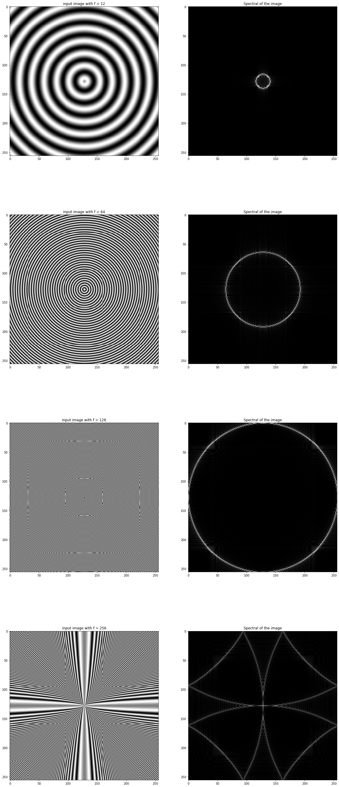
2.2: Spectral and Homomorphic Filtering
1) Visualize Image and Spectrum with Parasite Frequencies
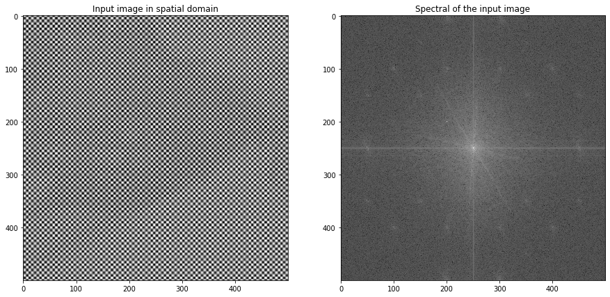
A mysterious file is provided, representing a famous portrait. Its identification is obscured by a double sinusoidal parasite signal at frequencies $\pm 50$ along each direction ($\pm x, \pm y$).
Task: Load the file imageMystere.png, display it and its Fourier Transform. To enhance visibility, display the spectrum in decibel scale.
Explanation:
Artificial images often have sparse spectral content, but real images (like the mysterious portrait) have dense spectra. To better visualize the parasite frequencies, the spectrum is shown in decibel scale. After applying fftshift, the center of the spectrum corresponds to frequency (0,0). The parasite signals appear as four bright points near the center at $\pm 50$.
1
2
3
4
5
6
7
8
9
10
11
12
13
14
15
16
17
18
img = cv2.imread('imageMystere.png', cv2.IMREAD_GRAYSCALE)  # Load image in grayscale
fft_img = np.fft.fft2(img) # Compute FFT of the image
spect_img_shift = abs(np.fft.fftshift(fft_img)) # Shifted FFT spectrum for visualization

# Display image and its spectrum side by side
fig1, (ax, ax1) = plt.subplots(1,2)
ax.imshow(img, vmin=0, vmax=255)
ax.set_title('Input image in spatial domain')

# Use log scale for spectrum to enhance visibility of frequencies
epsilon = 1e-7 # To avoid a log(0) error.
ax1.imshow(20*np.log10(spect_img_shift+epsilon))
ax1.set_title('Spectral of the input image')

# For better visualization, show spectrum in full size
plt.figure()
plt.imshow(20*np.log10(spect_img_shift+epsilon), vmin = 0, vmax = 255)
plt.title('Spectral of the image in the original size ')
Observation: The parasite signature is visible as four highlighted points around the center at frequencies $\pm 50$.
2) Construct and Apply Notch Filter in Fourier Domain
To eliminate the perturbations directly from the Fourier domain, we create a filter using multiple Gaussian profiles. The formula is:
\[H(u, v) = 1-e^{-((u \pm f)^2+(v \pm f)^2)/\sigma }\]where $\sigma$ tunes the selectivity and $f$ is the frequency to filter. By combining several Gaussian profiles centered at the parasite frequencies, we construct a mask that suppresses these unwanted components.
1
2
3
4
5
6
7
8
9
10
11
12
13
14
15
16
17
18
19
20
sigma = 5
x_size = fft_img.shape[0]
y_size = fft_img.shape[1]
x = np.arange(0,x_size)
y = np.arange(0,y_size)
u, v = np.meshgrid(x, y)

## Gaussian profiles
f = 50
G1 = np.exp(-(((u-f)**2)+(v-f)**2)/sigma)
G2 = np.exp(-(((u-(x_size-f))**2)+(v-f)**2)/sigma)
G3 = np.exp(-(((u-(x_size-f))**2)+(v-(y_size-f))**2)/sigma)
G4 = np.exp(-(((u-f)**2)+(v-(y_size-f))**2)/sigma)


H = 1- (G1+G2+G3+G4)
H_shift = np.fft.fftshift(H)

filtered_fft = H*fft_img # Filtering in frequency domain
Observation: The $\sigma$ value changes the standard deviation of the Gaussian profile. The filter $H$ acts as a band-stop (notch) filter, removing the single frequency at $\pm50$. Small $\sigma$ values create a narrow notch filter. Increasing $\sigma$ broadens the affected area, making the filter a wider band-stop. The Fourier spectrum will show black areas at the filtered frequencies, and the filter performs as a band-stop filter with higher bandwidth as $\sigma$ increases.
3) Reconstruct Filtered Image and Analyze Spectrum
After filtering the Fourier Transform with the mask (not just the magnitude), reconstruct the image using the inverse Fourier Transform. This step restores the spatial domain image with the perturbations removed.
1
2
3
4
5
6
7
8
9
filtered_img = np.fft.ifft2(filtered_fft)  # Inverse FFT to get filtered image in spatial domain
plt.imshow(abs(filtered_img))  # Display the filtered image
plt.show()

# Compute and display the FFT of the filtered image
fft_filtered_img = np.fft.fft2(filtered_img)
plt.imshow(20*np.log10(abs(np.fft.fftshift(fft_filtered_img))+epsilon), vmin = 0, vmax = 255)  # Log scale for spectrum
plt.title("The filtered image in Frequency domain with  $\sigma= {}$".format(sigma))
plt.show()
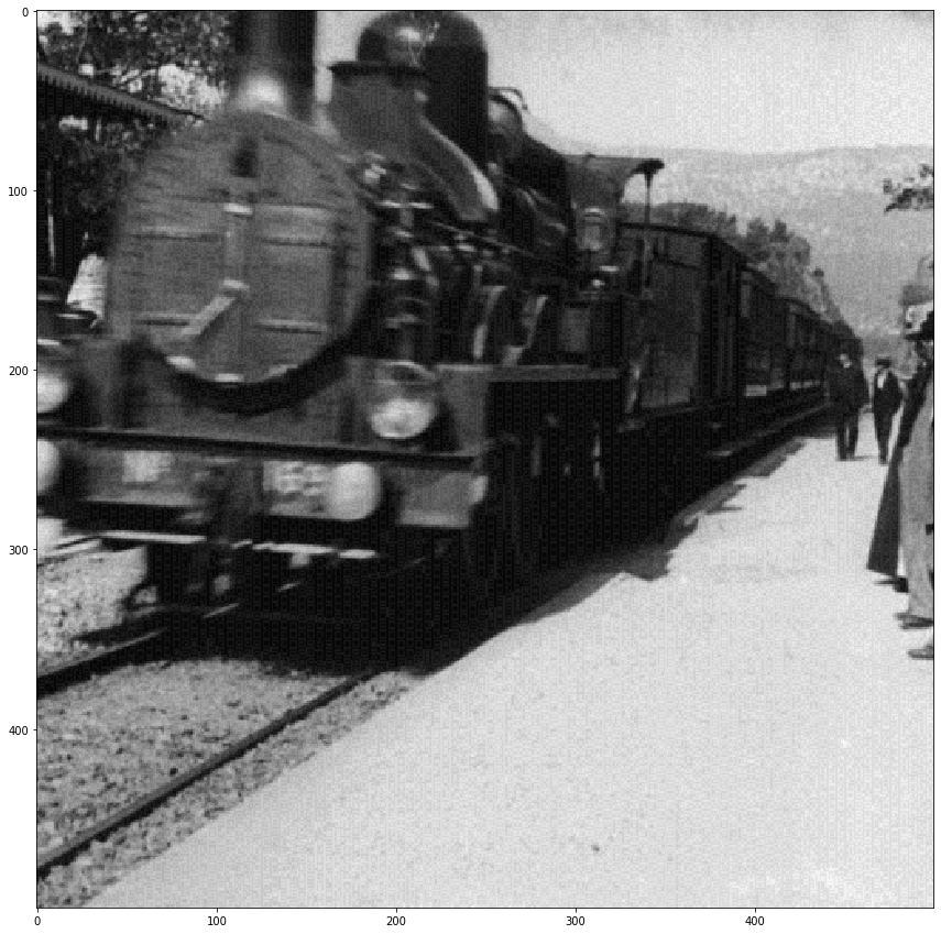
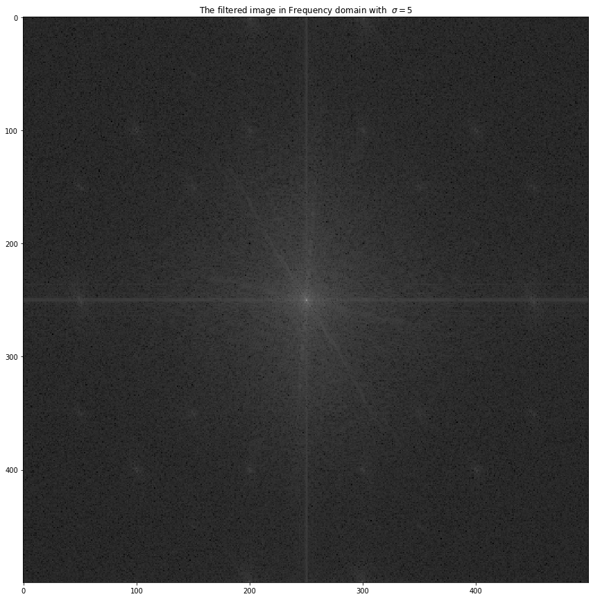
Observation: The reconstructed image has the parasite frequencies removed, and its spectrum shows the absence of the previously highlighted points. This demonstrates the effectiveness of frequency domain filtering for removing periodic noise.
4) Homomorphic Filtering for Illumination and Contrast Enhancement
The homomorphic filter is defined as:
$H(u, v)=(\gamma_H-\gamma_L)[1-e^{-c\frac{D^2(u, v)}{D^2_0}}]+\gamma_L$ where $D(u, v)=u^2+v^2$
This filter is applied to the Fourier Transform of the logarithmic image. After filtering, the result is exponentiated to return to the spatial domain.
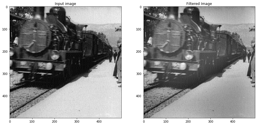
1
2
3
4
5
6
7
8
9
10
11
12
13
14
15
16
17
18
19
20
21
22
23
24
25
26
def homomorphic(u , v , img_size = (500,500) , gamma_l = 0.5, gamma_h = 2 , D_0 = 2 , c = 1):
    H = (gamma_h-gamma_l) * (1-np.exp(-c*((u-img_size[0]/2)**2+(v-img_size[1]/2)**2)/D_0**2)) + gamma_l
    return np.fft.fftshift(H)

# Apply homomorphic filtering
x = np.arange(0,x_size)
y = np.arange(0,y_size)
u, v = np.meshgrid(x, y)
homofilter = homomorphic(u, v, img_size=(x_size, y_size), gamma_l=0.5, gamma_h=2, D_0=2)
homofilter_shift = np.fft.fftshift(homofilter)
plt.figure()
plt.imshow(abs(homofilter_shift))
plt.title("Homomorphic Filter")

# Apply to log-image
img_log = np.log(filtered_img)
img_fft = np.fft.fft2(img_log)
filt_spectral = img_fft * homofilter

# Inverse FFT and exponentiate
filt_img_log = np.fft.ifft2(filt_spectral)
filt_img = np.exp(filt_img_log)
plt.figure()
plt.imshow(abs(filt_img))
plt.title("Homomorphic Filtered Image")
plt.show()
Observation: The homomorphic filter enhances reflectance (high frequencies) and suppresses illumination (low frequencies). $\gamma_H$ and $\gamma_L$ control the gain for high and low frequencies, while $D_0$ sets the cutoff frequency. The result is improved contrast and detail in the image.
Project repository
GitHub Code: Image Processing Project