Image processing: Segmentation (Part two)
Project && Guide
Table of Contents
- Overview
- Key Steps and Code Explanations
- 10. Median Filtering on Color Image
- 11. Extracting Unique Colors
- 12. Naive Posterization and Color Distance
- 13. Naive Posterization Result and Limitation
- 14. K-means Posterization
- 15. Channel-wise Posterization
- 16. HSV Color Space and Channel Ranges
- 17. HSV Channel Posterization and Color Counting
- 18. Adding Edges to Stylized Drawings
- 19. Improving Drawing Realism: Thinner and Colored Edges
- Project repository
Overview
This post explores advanced color image segmentation and artistic drawing effects using Python. The workflow includes:
- Median filtering for noise reduction on color images
- Color posterization using both naive (frequency-based) and k-means clustering approaches
- Channel-wise posterization to independently reduce the number of hues, saturations, and values
- Manipulation and analysis in the HSV color space
- Combining edge detection (gradient, Marr-Hildreth, Canny) with posterized color images to create stylized, drawing-like results
- Techniques to further enhance the realism of the drawing effect by refining edge thickness and coloring edges
Each step is explained with code and visualizations, demonstrating how color quantization and edge information can be combined for creative image transformations. The notebook is designed to help you understand and implement advanced segmentation and stylization pipelines for color images.
Key Steps and Code Explanations
10. Median Filtering on Color Image
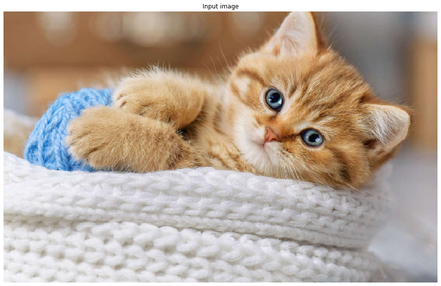
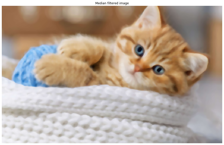
The input image is loaded, filtered with a median filter of size 9 to reduce noise, and displayed. This preprocessing step helps improve the quality of subsequent color segmentation.
1
2
3
4
img = cv2.imread('chaton.png')
img_med = cv2.medianBlur(img, 9)
imshow(img, title='Input image', is_bgr=True)
imshow(img_med, title='Median filtered image', is_bgr=True)
11. Extracting Unique Colors
To prepare for posterization, all unique colors in the image and their frequencies are extracted. This is the basis for reducing the color palette.
1
2
3
4
5
6
7
def recense_colors(img):
	if img.ndim == 3:
		unique_colors, count = np.unique(img.reshape(-1, img.shape[-1]), axis=0, return_counts=True)
	else:
		img_1_unique, count = np.unique(img, return_counts=True)
		unique_colors = img_1_unique.reshape(-1, 1)
	return unique_colors, count
12. Naive Posterization and Color Distance
Posterization reduces the number of colors by keeping only the K most frequent ones. The Euclidean distance is used to assign each pixel to its closest color in the reduced palette.
1
2
3
4
5
6
7
8
9
10
11
12
13
14
15
16
17
def euclidean_distance(col1, col2):
	"""
	Returns the table of all Euclidean distances between two color arrays.
	:param col1: Array of shape Nx3
	:param col2: Array of shape Mx3
	:return d: Array of shape NxM
	"""
	return scipy.spatial.distance.cdist(col1, col2, 'euclidean')

def naive_posterization(img, K=32):
	h, w, c = img.shape
	unique_colors, counts = recense_colors(img)
	T2 = unique_colors[np.argsort(counts)[-K:], :]
	distances = euclidean_distance(T2, img.reshape(-1, c))
	indices_d_min = np.argmin(distances, axis=0)
	posterization = T2[indices_d_min, :]
	return posterization.reshape(h, w, c)
13. Naive Posterization Result and Limitation
The result of naive posterization with K=64 is displayed. This method may miss important but infrequent colors.
1
2
img_naive_poster = naive_posterization(img_med, 64)
imshow(img_naive_poster, is_bgr=True)
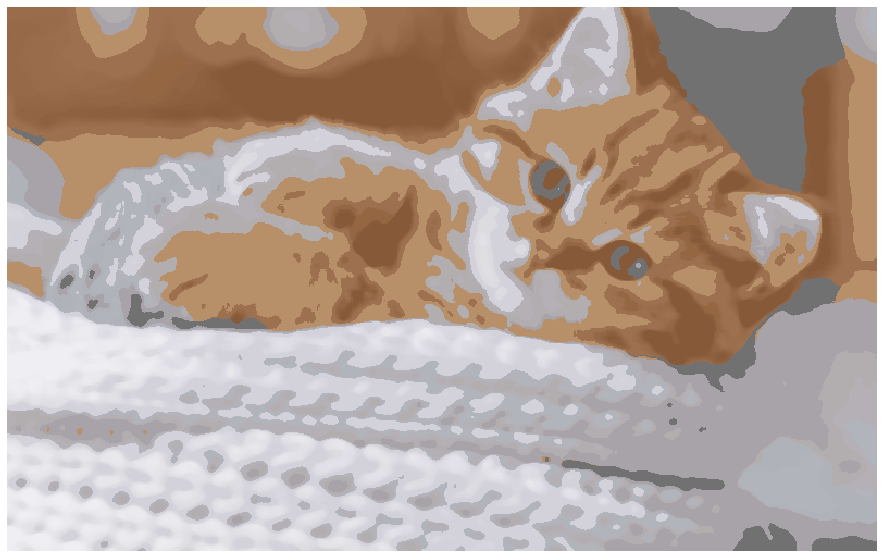
Limitation: Naive posterization only considers the most frequent colors, so rare but visually important colors may be omitted.
14. K-means Posterization
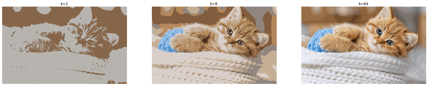
K-means clustering groups similar colors, providing a more representative reduced palette. The function below applies k-means to the unique colors and assigns each pixel to its cluster center.
1
2
3
4
5
6
7
8
def posterizations_kmeans(img, K=8):
	h, w, c = img.shape
	unique_colors, counts = recense_colors(img)
	T2 = f2int(kmeans(int2f(unique_colors), K)[0])
	distances = euclidean_distance(T2, img.reshape(-1, c))
	indices_d_min = np.argmin(distances, axis=0)
	posterization = T2[indices_d_min, :]
	return posterization.reshape(h, w, c)
1
2
3
4
5
6
7
fig1, (ax1, ax2, ax3) = plt.subplots(1, 3)
img_kmean_poster = posterizations_kmeans(img, 2)
imshow(img_kmean_poster, "k=2", is_bgr=True, ax=ax1)
img_kmean_poster = posterizations_kmeans(img, 8)
imshow(img_kmean_poster, "k=8", is_bgr=True, ax=ax2)
img_kmean_poster = posterizations_kmeans(img, 64)
imshow(img_kmean_poster, "k=64", is_bgr=True, ax=ax3)
Observation: K-means provides a better color summary, and increasing K makes the posterized image closer to the original.
15. Channel-wise Posterization
Instead of global color reduction, each channel (e.g., hue, saturation, value) can be posterized independently using k-means.
1
2
3
4
5
6
7
8
def posterize_grayscale(canal, K=8):
	h, w = canal.shape
	unique_colors, counts = recense_colors(canal)
	T2 = f2int(kmeans(int2f(unique_colors), K)[0])
	distances = euclidean_distance(T2, canal.reshape(-1, 1))
	indices_d_min = np.argmin(distances, axis=0)
	posterization = T2[indices_d_min, :]
	return posterization.reshape(h, w)
1
2
3
4
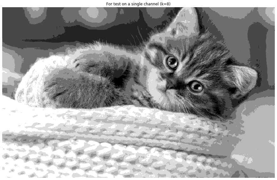
# Example: posterize the blue channel
img_gray = cv2.imread('chaton.png')[:, :, 0]
img_kmean_poster = posterize_grayscale(img_gray, 8)
imshow(img_kmean_poster, "For test on a single channel (k=8)")
16. HSV Color Space and Channel Ranges
We will use the HSV (Hue/Saturation/Value) color space, which is very similar to HSI. To convert between RGB and HSV, use:
1
2
hsv = cv2.cvtColor(rgb, cv2.COLOR_RGB2HSV)
rgb = cv2.cvtColor(hsv, cv2.COLOR_HSV2RGB)
Display the three channels H, S, and V separately and comment on their ranges.
Code:
1
2
3
4
5
6
7
8
9
10
11
img_hsv = cv2.cvtColor(img_med, cv2.COLOR_BGR2HSV)
fig1, (ax1, ax2, ax3) = plt.subplots(1, 3)
h = img_hsv[:, :, 0]
s = img_hsv[:, :, 1]
v = img_hsv[:, :, 2]
title_h = "The H channel is ranged between %.1f and %.1f" % (h.min(), h.max())
title_s = "The S channel is ranged between %.1f and %.1f" % (s.min(), s.max())
title_v = "The V channel is ranged between %.1f and %.1f" % (v.min(), v.max())
imshow(h, title=title_h, ax=ax1)
imshow(s, title=title_s, ax=ax2)
imshow(v, title=title_v, ax=ax3)
Explanation: The $H$ channel shows the colors, while $S$ and $V$ add saturation and value to each color. The variation of pixel values in the $H$ channel is greater compared to $S$ and $V$. Generally, $H$ ranges from 0 to 180, while $S$ and $V$ range from 0 to 255. The specific ranges are shown in the plot titles.
17. HSV Channel Posterization and Color Counting
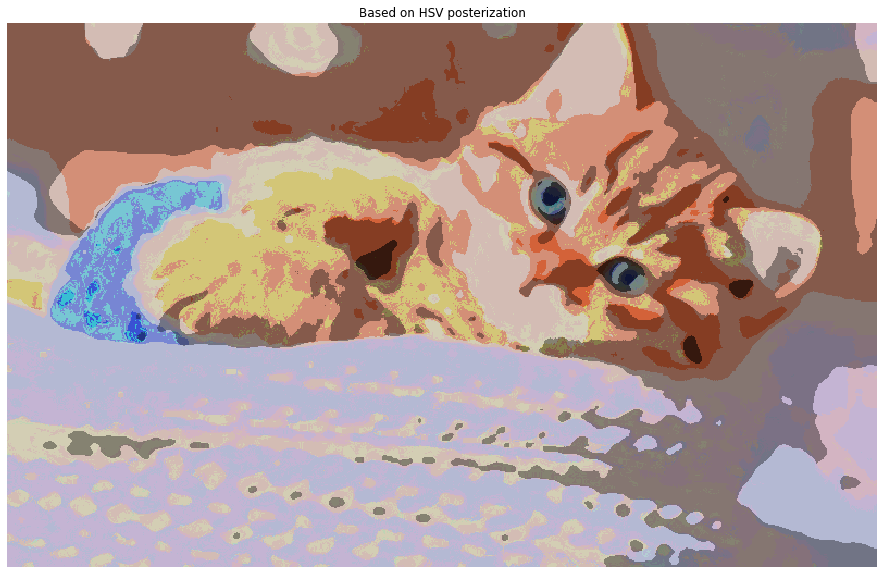
Posterize each channel of the HSV image independently so that:
- Hue contains 8 different values
- Saturation only 3
- Value only 3
Then, reconstruct the image in the RGB color space and display it. What is the theoretical maximum number of RGB colors under these constraints? How many unique colors are there after posterization?
Code:
1
2
3
4
5
6
7
8
9
10
11
12
hh, ww, cc = img_hsv.shape
h = img_hsv[:, :, 0]
h_post = posterize_grayscale(h, K=8).reshape(hh, ww, 1)
s = img_hsv[:, :, 1]
s_post = posterize_grayscale(s, K=3).reshape(hh, ww, 1)
v = img_hsv[:, :, 2]
v_post = posterize_grayscale(v, K=3).reshape(hh, ww, 1)
img_hsv_post = np.concatenate((h_post, s_post, v_post), axis=2)
img_rgb_post = cv2.cvtColor(img_hsv_post, cv2.COLOR_HSV2BGR)
num_of_color = recense_colors(img_rgb_post)[0].shape[0]
print("The number of unique colors in the posterized image is %d" % num_of_color)
imshow(img_rgb_post, title="Based on HSV posterization", is_bgr=True)
Explanation:
Theoretically, $8 \times 3 \times 3 = 72$ different colors can be produced based on the posterization levels of each channel. However, in practice, the number of unique colors in the posterized image may be lower due to overlapping or unused color combinations. In this example, there are 48 unique colors in the posterized image (as determined by the recense_colors function).
18. Adding Edges to Stylized Drawings
Let’s finish our drawing by adding edges! We will use the ones obtained in the first part.
To do so, you have many options: indexation (set to 0 the colors of the images in the edges), piecewise multiplication, bitwise_xor… You’re free to choose the approach you like the most!
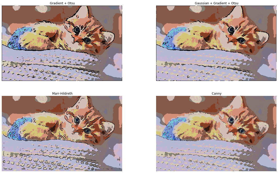
Create four subplots and display the different edges (gradients, canny, LoG…) in black on top of the posterized image from previous question. Which one seems the most convincing for our application?
Code:
1
2
3
4
5
6
7
8
9
10
11
12
13
14
15
16
17
18
fig1, ((ax1, ax2),(ax3, ax4)) = plt.subplots(2,2, figsize=(20,12))

img_rgb_post_grad = img_rgb_post*1
img_rgb_post_gauss_grad = img_rgb_post*1
img_rgb_post_Marr = img_rgb_post*1
img_rgb_post_canny = img_rgb_post*1

img_rgb_post_grad[img_grad_b,:]=0
imshow(img_rgb_post_grad,title=' Gradient + Otsu', is_bgr=True, ax = ax1)

img_rgb_post_gauss_grad[img_gauss_grad_b,:]=0
imshow(img_rgb_post_gauss_grad,title=' Gaussian + Gradient + Otsu', is_bgr=True, ax=ax2)

img_rgb_post_Marr[img_zero,:]=0
imshow(img_rgb_post_Marr,title=' Marr-Hildreth', is_bgr=True, ax = ax3)

img_rgb_post_canny[img_canny,:]=0
imshow(img_rgb_post_canny,title=' Canny', is_bgr=True, ax = ax4)
Explanation: In this step, it seems that $Gaussian + Gradient + Otsu$ approach can detect the cat edges without highlighting unnecessary contours. Therefore, based on our opinion, although the method is not the most sophisticated one, it creates the most convincing image. Moreover, by further processing, Canny approach seems to provide the most appropriate output since it gives consistent and thin edges.
19. Improving Drawing Realism: Thinner and Colored Edges
In reality, most lines of a drawing are rarely perfectly black; their colors may depend on their widths and the colors of the object they delimit.
By taking into account these two considerations, propose a way to improve our drawing effect. You can combine as you want any of our previously obtained results.
Explanation: The first problem is the thickness of the extracted edges during our edge detection algorithm. To have thinner edges, the morphological operation erosion (or opening) applied on the binary edge image can be an option. To apply another improvement, some other modifications (a combination of morphological operations) can be used to remove the spur pixels remaining from previous thinning operation.
The second problem is unrealistic black edges. To deal with this issue, one can mask the binary image with the original one to transfer the local specific colors from background to the edges, then a colored edge image is obtained. It should be highlighted in the main image by adding these two images together. imshow(s, title=title_s, ax=ax2)
1
2
3
v = img_hsv[:, :, 2]
title_v = "The V channel is ranged between %.1f and %.1f" % (v.min(), v.max())
imshow(v, title=title_v, ax=ax3)
Observation: H ranges from 0 to 180, S and V from 0 to 255. H encodes color, S and V encode saturation and brightness.
Project repository
GitHub Code: Image Processing Project