Image processing: Segmentation (Part one)

Project && Guide

Table of Contents

• Overview
• Key Steps and Code Explanations
  • Library Imports and Utility Functions
  • 1. Load and Display Input Image
  • 2. Compute and Display Lightness
  • 3. Median Filtering
  • 4. Gradient Computation (Perwitt Filters)
  • 5. Gaussian Filtering and Gradient
  • 6. Otsu Thresholding Function
  • 7. Marr-Hildreth (Laplacian of Gaussian) Edge Detection
  • 8. Canny Edge Detection
  • 9. Comparison of Edge Detection Methods
  • Project repository

Overview

This post provides a comprehensive walkthrough of image segmentation using Python libraries including OpenCV, NumPy, SciPy, and Matplotlib. The workflow covers:

• Loading and preprocessing images
• Computing lightness and applying median and Gaussian filtering to reduce noise
• Extracting edges using gradient-based methods (Perwitt filters), Marr-Hildreth (Laplacian of Gaussian), and Canny edge detection
• Applying Otsu’s thresholding for automatic binarization
• Comparing the effectiveness of different edge detection techniques

Each step is explained with code and visualizations, highlighting the impact of various filters and parameters on segmentation results. The notebook is designed to help you understand and implement practical image segmentation pipelines for a variety of applications.

Key Steps and Code Explanations

Library Imports and Utility Functions

The following code imports essential libraries for image processing and visualization, and defines utility functions for displaying images and converting between float and integer formats. These utilities are used throughout the segmentation workflow.

import cv2  # OpenCV for image operations
import numpy as np  # Numerical operations
import scipy  # Scientific computing
import matplotlib.pyplot as plt  # Plotting
plt.rcParams['image.cmap'] = 'gray'  # Set default colormap to grayscale
import matplotlib
import scipy.signal as signal  # Signal processing functions
matplotlib.rcParams['figure.figsize'] = (25.0, 10.0)  # Set default figure size
from scipy.cluster.vq import kmeans  # K-means clustering

def imshow(img, title=None, ax=None, is_bgr=False, cmap='gray'):
    """
    Display an image with optional title and color map.
    img: image to display (hxw or hxwx3)
    title: Figure's title
    ax: Axis to display on (optional)
    is_bgr: Convert BGR to RGB if True
    cmap: Color map
    """
    show=False
    plt.axis('off')
    if ax is None:
        show=True
        if title is not None:
            plt.title(title)
        ax = plt
    else:
        if title is not None:
            ax.set_title(title)
            ax.set_axis_off()
    if img.ndim==2:
        ax.imshow(img, cmap='gray')
    else:
        if is_bgr:
            img = img[:,:,::-1].copy()
        ax.imshow(img)
    if show:
        plt.show()

def f2int(img):
    return (img*255).astype(np.uint8)

def int2f(img):
    return img.astype(np.float32)/255.

1. Load and Display Input Image

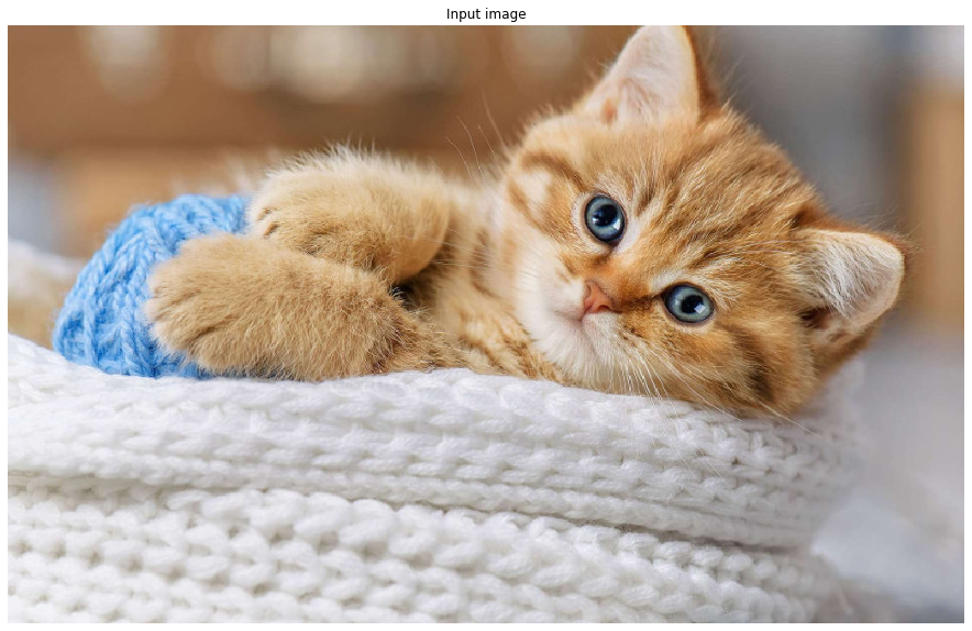
This section loads the input image from disk, converts it to a floating-point format for processing, and displays it using the utility function defined above.

img = int2f(cv2.imread('chaton.png'))  # Read image and convert to float
imshow(img, title='Input image', is_bgr=True)  # Show image with title

2. Compute and Display Lightness

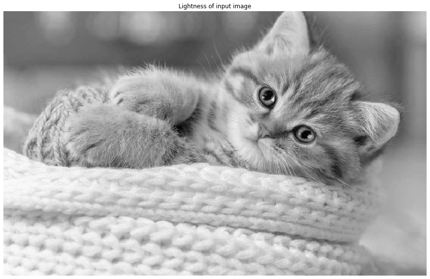
Here, the lightness channel of the image is computed by averaging the maximum and minimum values across the RGB channels. This reduces the color image to a single-channel grayscale image, simplifying further processing.

img_light = 0.5 * (img.max(2) + img.min(2))  # Calculate lightness from max and min RGB values
imshow(img_light, title='Lightness of input image')  # Show lightness image

3. Median Filtering

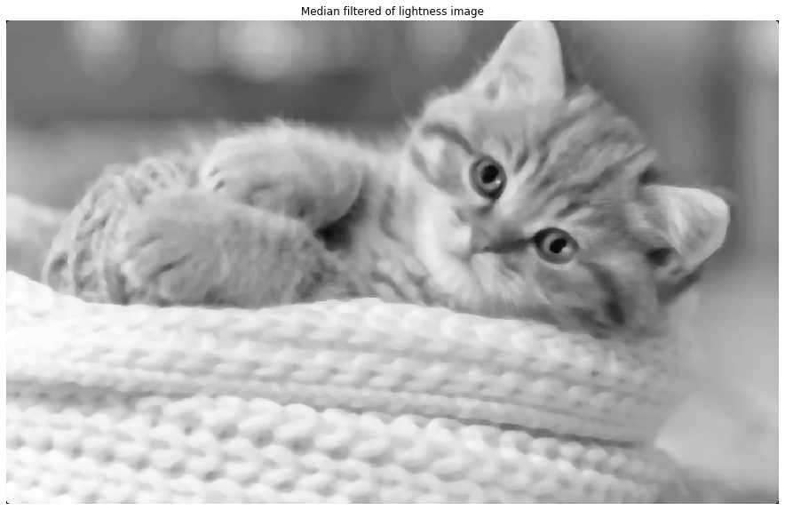
This code applies a median filter to the lightness image to reduce noise and smooth out small variations, which helps improve the quality of subsequent segmentation steps.

kernel_size = 7  # Size of the median filter
img_light = signal.medfilt2d(img_light, kernel_size)  # Apply median filter
imshow(img_light, title='Median filtered of lightness image')  # Show filtered image

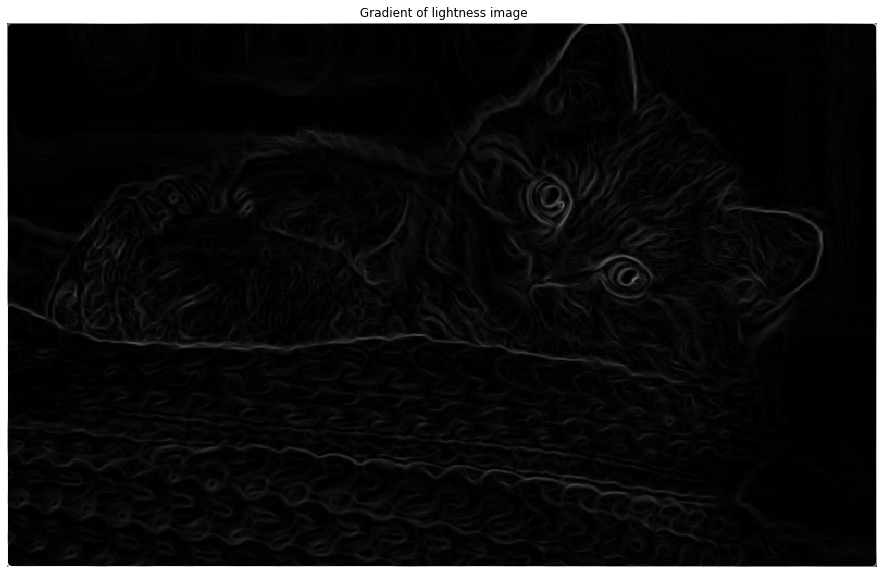
4. Gradient Computation (Perwitt Filters)

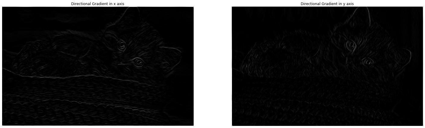
This section computes the image gradients using Perwitt filters in both the x and y directions. The gradients highlight edges and transitions, which are important features for segmenting different regions in the image.

fig1, (ax1, ax2) = plt.subplots(1,2)
g_x = [[1., 1., 1.], [0, 0, 0], [-1., -1., -1.]]  # Perwitt filter for x direction
x_grad = signal.convolve2d(img_light, g_x, mode='same')  # Compute x gradient
imshow(abs(x_grad), title='Directional Gradient in x axis', ax=ax1)
g_y = [[1., 0, -1], [1, 0, -1.], [1, 0, -1.]]  # Perwitt filter for y direction
y_grad = signal.convolve2d(img_light, g_y, mode='same')  # Compute y gradient
imshow(abs(y_grad), title='Directional Gradient in y axis', ax=ax2)
plt.show()
img_grad = np.sqrt(x_grad**2 + y_grad**2)  # Compute gradient magnitude
imshow(img_grad, title='Gradient of lightness image')

5. Gaussian Filtering and Gradient

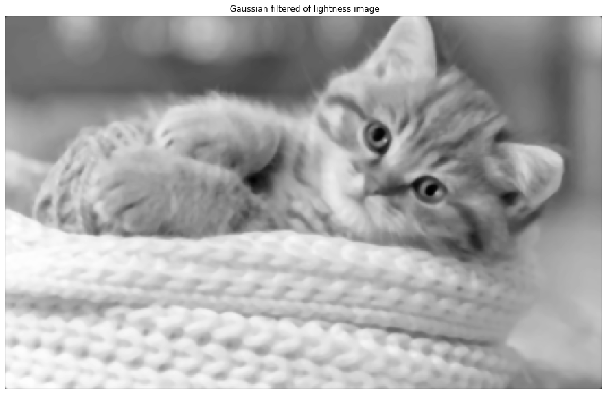
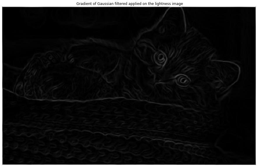
This part applies a Gaussian filter to the lightness image for further smoothing, then recomputes the gradients. Smoothing with a Gaussian kernel helps reduce noise and makes edge detection more robust.

kernel_gauss = create_gauss_kernel(size=5, sigma=1)  # Create Gaussian kernel
img_gauss = signal.convolve2d(img_light, kernel_gauss, mode='same')  # Apply Gaussian filter
g_x = [[1., 1., 1.], [0, 0, 0], [-1., -1., -1.]]
g_y = [[1., 0, -1], [1., 0, -1.], [1., 0, -1.]]
x_grad = signal.convolve2d(img_gauss, g_x, mode='same')
y_grad = signal.convolve2d(img_gauss, g_y, mode='same')
img_gauss_grad = np.sqrt(x_grad**2 + y_grad**2)
imshow(img_gauss, title='Gaussian filtered of lightness image')
imshow(img_gauss_grad, title='Gradient of Gaussian filtered applied on the lightness image')

6. Otsu Thresholding Function

The following function implements Otsu’s method, which automatically determines an optimal threshold value for segmenting an image into foreground and background. This is a crucial step for many segmentation tasks.

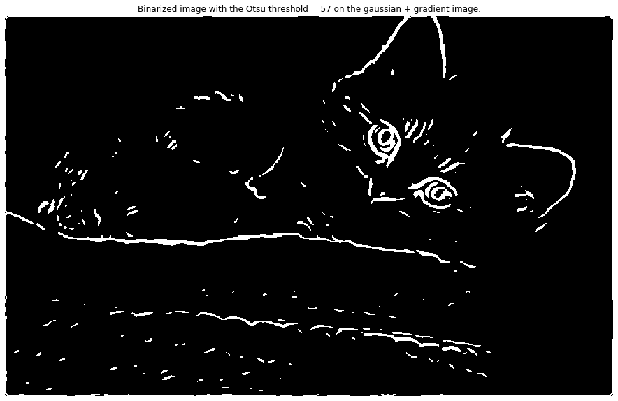
Applying Otsu Thresholding and Binarization

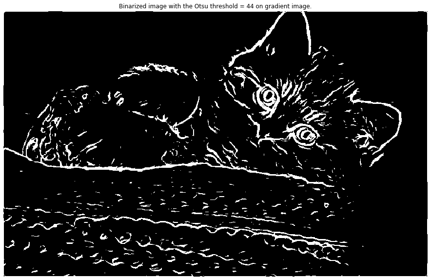
After defining the Otsu thresholding function, the next step is to apply it to gradient images for binarization. The gradients and Gaussian-filtered gradients are converted to integer format and thresholded using Otsu’s method. For comparison, OpenCV’s built-in Otsu thresholding is also used. The results are visualized to show the effect of thresholding on edge detection and segmentation.

The code below demonstrates:

• Computing Otsu thresholds for gradient and Gaussian-filtered gradient images
• Binarizing these images using the computed thresholds
• Comparing the custom Otsu threshold with OpenCV’s built-in function
• Visualizing the binarized results

def otsu_thresholding(img):
    assert img.dtype == np.uint8, "The image must have a uint8 type"
    thresholds = np.unique(img)
    hist, bins = np.histogram(img, np.arange(256))
    bins = bins[:-1]
    hist = hist / img.size
    nu = 0
    for k in thresholds:
        hist_c1 = hist[:k+1]
        hist_c2 = hist[k+1:]
        P1_k = hist_c1.sum() / hist.sum()
        P2_k = hist_c2.sum() / hist.sum()
        if P1_k == 0:
            continue
        if P2_k == 0:
            break
        m1_k = np.sum(bins[:k+1] * hist_c1) / P1_k.astype(np.float32)
        m2_k = np.sum(bins[k+1:] * hist_c2) / P2_k.astype(np.float32)
        var_interclasse = P1_k * P2_k * (m2_k - m1_k) ** 2
        if var_interclasse > nu:
            threshold = k
            nu = var_interclasse
    thresholded = threshold
    return thresholded

# Apply Otsu thresholding to gradient images
thr_grad = otsu_thresholding(f2int(img_grad))  # Image taken from Q4
thr_gauss_grad = otsu_thresholding(f2int(img_gauss_grad))  # Image taken from Q5

# Binarize the images
img_grad_b = f2int(img_grad) > thr_grad
img_gauss_grad_b = f2int(img_gauss_grad) > thr_gauss_grad

# Compare with OpenCV's built-in Otsu thresholding
ret2, th2 = cv2.threshold(f2int(img_gauss_grad), 0, 255, cv2.THRESH_OTSU)
print('For test:\nThreshold using our function is %d.\nThreshold using cv2 function is %d.' % (thr_gauss_grad, ret2))

# Visualize the results
imshow(img_grad_b, title='Binarized image with the Otsu threshold = {} on gradient image.'.format(thr_grad))
imshow(img_gauss_grad_b, title='Binarized image with the Otsu threshold = {} on the gaussian + gradient image.'.format(thr_gauss_grad))

7. Marr-Hildreth (Laplacian of Gaussian) Edge Detection

This section explores edge detection using the Marr-Hildreth approach, also known as the Laplacian of Gaussian (LoG) method. The process involves:

• Smoothing the image with a Gaussian filter to reduce noise.
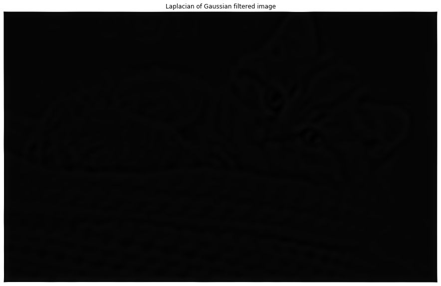
• Computing the Laplacian (second derivative) of the smoothed image to highlight regions of rapid intensity change.
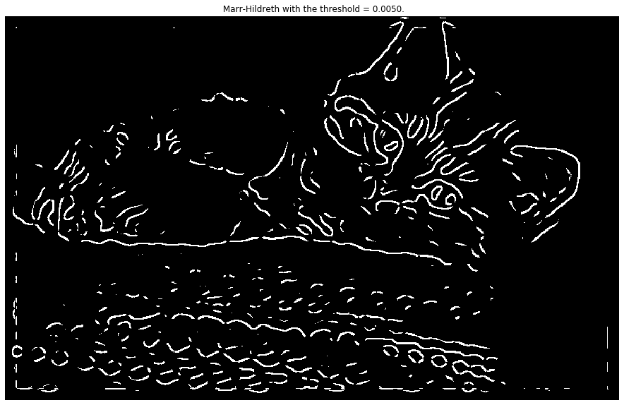
• Detecting edges by finding zero-crossings in the Laplacian image, with a threshold to filter out weak edges.

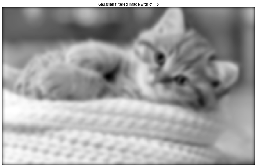
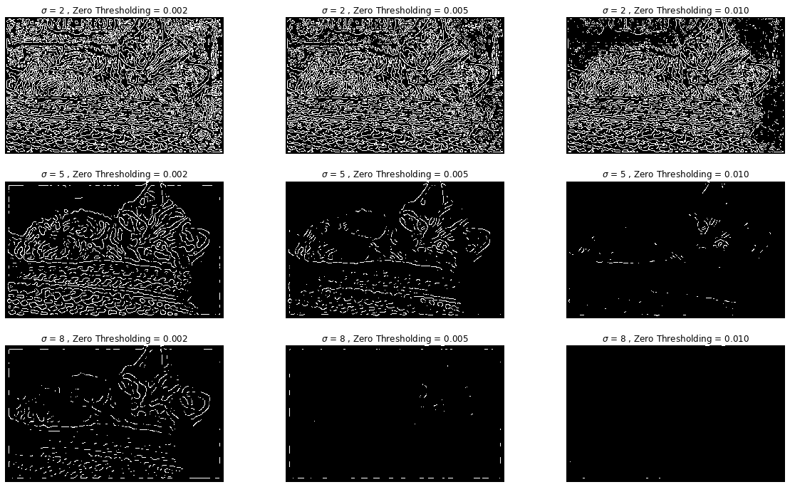
By varying the Gaussian standard deviation ($\sigma$) and the zero-crossing threshold, you can control the sensitivity and thickness of detected edges. Larger $\sigma$ values produce smoother images and less noisy edges, while higher thresholds reduce the number of detected edges.

This method is effective for detecting closed contours and is less sensitive to noise than simple gradient-based methods, but the choice of parameters significantly affects the results.

Implementation and Parameter Exploration

The following code demonstrates the Marr-Hildreth edge detection process, including parameter exploration for $\sigma$ and the zero-crossing threshold:

# Function to detect zero-crossings in the Laplacian image
def zeros_crossing(img, threshold):
    out = np.zeros_like(img)
    for i in range(1, img.shape[0]-1):
        for j in range(1, img.shape[1]-1):
            ec = 0
            if img[i-1, j]*img[i+1, j] < 0: # y direction
                ec = max(ec, np.abs(img[i+1, j]-img[i-1, j]))
            if img[i, j-1]*img[i, j+1] < 0: # x direction
                ec = max(ec, np.abs(img[i, j+1]-img[i, j-1]))
            if img[i-1, j-1]*img[i+1, j+1] < 0: # diagonal
                ec = max(ec, np.abs(img[i+1, j+1]-img[i-1, j-1]))
            if img[i+1, j-1]*img[i-1, j+1] < 0: # other diagonal
                ec = max(ec, np.abs(img[i+1, j-1]-img[i-1, j+1]))
            out[i, j] = ec
    threshold = threshold * np.max(out)
    return out > threshold

# Example: single parameter set
sigma_val = 5
kernel_gauss = create_gauss_kernel(size=6*sigma_val-1, sigma=sigma_val) # Gaussian Mask
img_gauss = signal.convolve2d(img_light, kernel_gauss, mode='same')
imshow(img_gauss, 'Gaussian filtered image with $\sigma$ = %d' % sigma_val)

mask_laplacian = np.asarray([[-1.,-1.,-1.], [-1.,8.,-1.], [-1.,-1.,-1.]]) # Laplacian mask
img_gauss_laplac = signal.convolve2d(img_gauss, mask_laplacian, mode='same')
imshow(img_gauss_laplac, 'Laplacian of Gaussian filtered image')

zero_thresh = 0.005
img_zero = zeros_crossing(img_gauss_laplac, zero_thresh)
imshow(img_zero, 'Marr-Hildreth with the threshold = %.4f.' % zero_thresh)

# Parameter exploration: different sigma and threshold values
fig1, ((ax0, ax1, ax2), (ax3,ax4,ax5),(ax6,ax7,ax8)) = plt.subplots(3,3,figsize = (20,12))
AX = [[ax0,ax1,ax2],[ax3,ax4,ax5],[ax6,ax7,ax8]]
SIGMA = [2, 5, 8]
THRESH = [0.002, 0.005, 0.01]
for i, sigma in enumerate(SIGMA):
    for j, thresh in enumerate(THRESH):
        kernel_gauss = create_gauss_kernel(size=6*sigma-1, sigma=sigma)
        img_gauss = signal.convolve2d(img_light, kernel_gauss, mode='same')
        img_gauss_laplac = signal.convolve2d(img_gauss, mask_laplacian, mode='same')
        img_zero_ = zeros_crossing(img_gauss_laplac, thresh)
        title = '$\sigma$ = %d , Zero Thresholding = %.3f'%(sigma, thresh)
        imshow(img_zero_, title = title, ax = AX[i][j])

Observations

By increasing the $\sigma$ value, the Gaussian filtered image becomes smoother and the detected edges are less noisy, but some fine details may be lost. Increasing the zero-crossing threshold reduces the number of detected edges, making the result sparser. Adjusting both parameters is important for accurate edge detection using the Marr-Hildreth method.

8. Canny Edge Detection

This section demonstrates edge detection using the Canny method, a widely used algorithm that detects a wide range of edges in images. The Canny method uses two thresholds (lower and upper) to identify strong and weak edges, and includes non-maximum suppression and edge tracking by hysteresis.

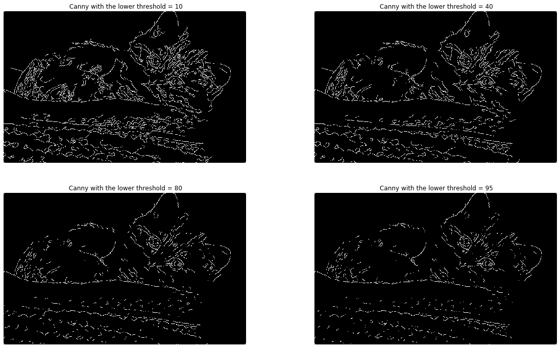
The following code applies the Canny edge detector to the lightness image, varying the lower threshold while keeping the upper threshold fixed at 100. The results show how the choice of thresholds affects the number and continuity of detected edges.

max_hysteresis = 100
min_hysteresis = 95
img_canny = cv2.Canny(f2int(img_light), min_hysteresis, max_hysteresis).astype(bool)

fig1, ((ax1, ax2),(ax3, ax4)) = plt.subplots(2,2, figsize=(20,12))
min_hysteresis = 10
imshow(cv2.Canny(f2int(img_light), min_hysteresis, max_hysteresis).astype(bool), title='Canny with the lower threshold = %d' % min_hysteresis, ax=ax1)
min_hysteresis = 40
imshow(cv2.Canny(f2int(img_light), min_hysteresis, max_hysteresis).astype(bool), title='Canny with the lower threshold = %d' % min_hysteresis, ax=ax2)
min_hysteresis = 80
imshow(cv2.Canny(f2int(img_light), min_hysteresis, max_hysteresis).astype(bool), title='Canny with the lower threshold = %d' % min_hysteresis, ax=ax3)
min_hysteresis = 95
imshow(cv2.Canny(f2int(img_light), min_hysteresis, max_hysteresis).astype(bool), title='Canny with the lower threshold = %d' % min_hysteresis, ax=ax4)

Observation: Increasing the lower threshold reduces the number of detected edges, resulting in fewer, more connected edge pixels. The Canny method provides thin and well-connected edges, and is less sensitive to noise compared to simple gradient-based methods.

9. Comparison of Edge Detection Methods

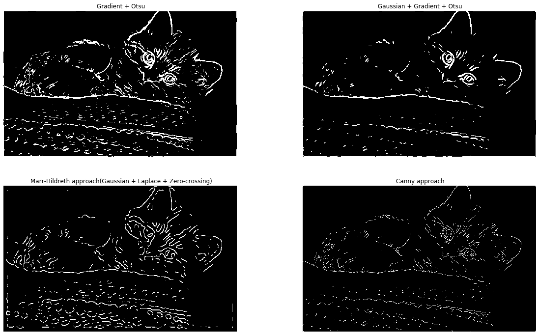
This section compares the results of four edge detection approaches: Gradient + Otsu, Gaussian + Gradient + Otsu, Marr-Hildreth (LoG), and Canny. The following code displays the results side by side for visual comparison.

fig1, ((ax1, ax2),(ax3, ax4)) = plt.subplots(2,2, figsize=(20,12))
imshow(img_grad_b, title='Gradient + Otsu', ax=ax1)
imshow(img_gauss_grad_b, title='Gaussian + Gradient + Otsu', ax=ax2)
imshow(img_zero, title='Marr-Hildreth approach (Gaussian + Laplace + Zero-crossing)', ax=ax3)
imshow(img_canny, title='Canny approach', ax=ax4)

Observation:

• Adding a Gaussian filter before gradient-based edge detection reduces noise and produces cleaner edges.
• The Canny method yields the thinnest and most consistent edges.
• The Marr-Hildreth approach is sensitive to the zero-crossing threshold, while the Canny method is less sensitive to the lower threshold.
• Overall, the Canny and Gaussian + Gradient + Otsu methods provide the most visually convincing results for edge detection in this context.

Project repository

GitHub Code: Image Processing Project